Book review: Image analysis and classification through image pre-processing and deep learning ANNs
By Shalin Hai-Jew, Kansas State University
Deep Learning-Based Image Analysis Under Constrained and Unconstrained Environments
Alex Noel Joseph Raj, Vijayalakshmi G.V. Mahesh, and Ruban Nersisson
IGI Global
2021
381 pp.
Once an innovation has been created and publicized, there has to be uptake of that innovation before there is practical impact. This is so, too, with deep learning through artificial neural networks, which stand to advance work in various domains and disciplines. Alex Noel Joseph Raj, Vijayalakshmi G.V. Mahesh, and Ruban Nersisson’s Deep Learning-Based Image Analysis Under Constrained and Unconstrained Environments (2021) provides an overview of various deep learning techniques applied to image analysis in healthcare and disease diagnosis, human emotion recognition, plant disease recognition, “ethnicity” recognition, optical character recognition (OCR) of handwriting, and other mainstream practical contexts. The respective chapters here show varying value in application, and at least one is fairly concerning in terms of possible societal mis-use.
“Deep learning” (or “deep structured learning”) refers to machine learning achieved through artificial neural networks, and the “deep” refers to the respective layers of the ANNs.
In these cases, the ANNs enable computers to identify more nuanced features of images that may reveal what category they may belong to even if what is exactly going on in the “hidden” layers of the ANNs may not be fully explicated. ANNs may learn from labeled data (supervised machine learning) or unlabeled data (unsupervised machine learning). Deep learning (also referred to as “deep neural learning” or “deep neural network”) is a subset of machine learning in artificial intelligence (AI).
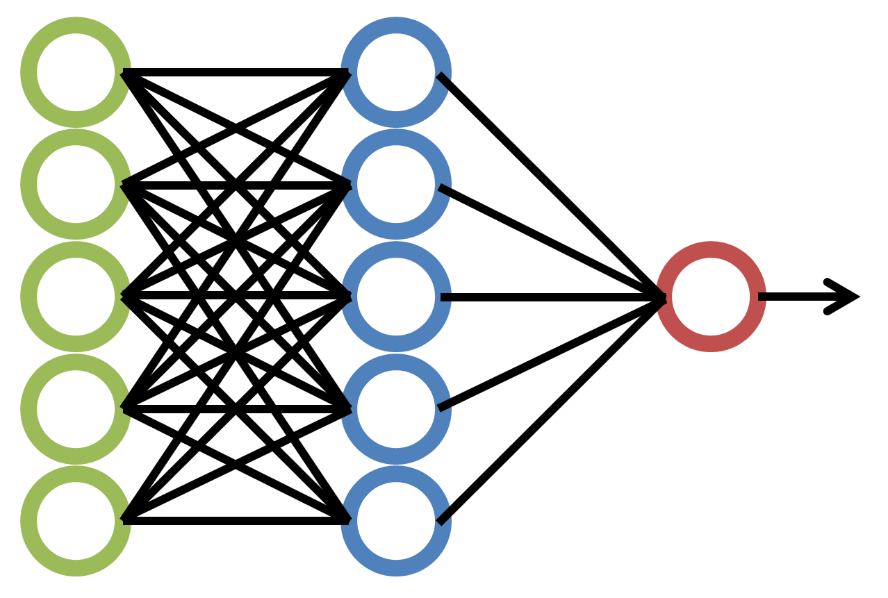
Deep learning is a subset of machine learning in artificial intelligence that has networks capable of learning unsupervised from data that is unstructured or unlabeled, and it can learn in other ways, too. ANNs were conceptualized decades ago as a sort of biomimetic version of animal neurons with inputs, complex interrelated processing, and outputs for awareness and decision-making and actions.
Figure 1. Artificial Neural Network (by Loxaxs on January 2018)
Images may be digitized from physical media (photos, x-rays, documents, and so on). They can be captured using various cameras, sensors, scanners, and other instruments. Their acquisition affects how the visual presents visually. Digital images may be pre-processed to heighten their readiness to be computationally analyzed and emplaced into different categories (often with high accuracy). A “constrained” context is one in which the visuals are delimited based on particular features; an “unconstrained” context is one in the “wild” in which the visuals are not delimited and may include high levels of noise and distractors for the digital image processing.
The first chapter of this collection focuses on the basics of a digital image. Chandra Prabha R. and Shilpa Hiremath’s “Computer Processing of an Image: An Introduction” (Ch. 1) differentiates digital images by type: binary, grayscale, color, indexed, and then various image format types (.gif, .jpg, JPEG 2000, .png, .tif, and .psd). “Analog” images are defined as having “a continuous range of values representing position and intensity” and digital ones comprised of spatial coordinates (on x and y axes) and different intensities of points at various locations on that two-dimensional plane (p. 2). “Digital” images can be binary (only two pixel levels of a 0 or a 1, black or white); grayscale as having values from 0 to 255 with different variations on gray (often used “in the medical and astronomy field(s)” (p. 3); a color image (in red, green, and blue or “RGB” or a “three-band monochrome image” and image information stored “in the form of a grey level in each spectral band” (p. 4); and indexed image where the image “has pixel values and a colormap value” where each pixel location is mapped to the colormap (p. 4).
As with many issues solved computationally, the challenge is disaggregated into various smaller parts and worked separately. There has to be computational knowledge as well as specialist knowledge of the issue at hand in the particular domain. Oftentimes, this means a cross-functional team collaborates. The general process of image analysis includes initial pre-processing (in some cases), identifying and locating the parts of an image of interest, verifying object identity, and categorizing the visuals. Under the covers, there are various subprocesses and parameters. The innovation here involves cobbling (engineering) various capabilities and systems for desired outcomes (proper classifying, most often).
Computer vision is built somewhat as an emulation of animal visual systems, with a cornea, pupil, lens, and retina working of a piece to enable sight information to be communicated through the optic nerve and into the brain (R. & Hiremath, 2021, p. 7). There are computational equivalents of dark adaptation (~ to a person entering a dark room from a bright-lit area and having their eyes adjust and adapt), and light adaptation (~ to a person entering a bright-lit space from a dark one and having their eyes adapt). Digital sensors serve as “the transduction process of a biological eye” where the human eyes’ rod and cone receptors “work in combination with ganglion cells to convert photons into an electrochemical signal which is the occipital lobe in our brain, and then this signal is processed in our brain. In the case of an image sensor, though photons are captured as charge electrons in silicon which is the sensing material and converted to a voltage value through the use of capacitors and amplifiers then later transferred into digital code which can be processed by a computer” (p. 9). Digital image analysis systems can take inputs from single sensors, line sensors, and array sensors (p. 9).
The co-authors offer an important list of definitions to understand terminology in this space, including “wavelets and multiresolution processing,” “compression,” “morphological processing,” “segmentation,” and others (R. & Hiremath, 2021, p. 10), as defined in the research literature. One such explanation follows:
Oversampling or up-sampling involves sampling “the signal more than the level which is set by Nyquist” and can improve the resolution of the image (p. 14). Undersampling involves “a band pass-filtered signal at a sample rate below its Nyquist rate” (p. 14). Images can be represented as a two-dimensional function f(x,y) where x and y are spatial coordinates on a two-dimensional plane and various amplitudes are represented in the various locales (p. 15). In these cases and the others in the text, spatial resolution (pixels or “picture elements” per square inch), color depth (bit depth), and such as important.
Naralasetty Niharika, Sakshi Patel, Bharath K.P., Balaji Subramanian, and Rajesh Kumar M.’s “Brain Tumor Detection and Classification Based on Histogram Equalization Using Machine Learning” (Ch. 2) opens by explaining the importance of discerning between benign and malignant brain tumors as early as possible when brain tissue starts to change. There are ways to evaluate a potential tumor based on different levels of “hardness”: Grade 1 (pilocytic astrocytoma) or the “least dangerous tumor,” Grade 2 (low grade astrocytoma), Grade 3 (anaplastic astrocytoma), and Grade 4 (glioblastoma) or “malignant and dangerous tumor” (p. 25). Their approach uses histogram equalization to change the gamma values (luminance) to raise the intensity of the tumor for heightened detection. Then, they use k-means clustering and Gaussian mixture model to segment the images to identify areas of interest. They use discrete wavelet transforms to extract features. They run a principal component analysis (PCA) to reduce features. Then, ultimately, they run a support vector machine (SVM) and artificial neural networks (ANNs) to conduct the classification (p. 23). Succinctly, the sequence reads: input image, histogram equalization, clustering (first k-means and then GMM), feature extraction, feature reduction, and classifier (first ANN and then SVM) (p. 26). Each sequential step contributes to the overall process of computational discernment.
A key to their sequence is histogram equalization, which is a method for “modifying image intensities to improve contrast.” There are different methods: “local histogram equalization, global histogram equalization, brightness preserving bi-histogram equalization, dualistic sub-image histogram equalization, recursive sub-image histogram equalization, (and) recursive mean separate histogram equalization (Niharika, Patel, K.P., Subramanian, & M., 2021, p. 27). Their approach is tested for accuracy, to control against false positives and false negatives.
Strivathsav Ashwin Ramamoorthy and Varun P. Gopi’s “Breast Ultrasound Image Processing” (Ch. 3) presents a case of “computer-aided diagnosis” (CAD) to support the work of radiologists assessing ultrasound imagery. In this work, the designed sequence involves the following steps in the analytical sequence: “pre-processing, segmentation, feature extraction, and classification” (p. 44). In this domain, early detection enables various health interventions that can keep the cancer from spreading further. However, ultrasound images (created from high frequency sound waves through the human tissue) tend to be low-contrast (without sufficient differences between light and dark) even as there are differences in densities between the cancer and healthy tissue. Various transforms enable visual enhancement of digital imagery for select details such as “contrast stretching, window slicing, and histogram modelling” (p. 45). “Histogram equalization and linear contrast stretching” is done automatically in this case (p. 45).
They explain the importance of image segmentation in the medical image analysis space:
“Fuzzification” refers to the ability to broaden “membership” of various objects to a particular set, instead of just going with a binary membership sense (in or out, 1 or 0). In this work, the work sequence involves normalizing the image given the narrow range of intensities (p. 46), fuzzifying the image (or representing the various degrees of truth in the image) (p. 47), capturing edge and textural information, enhancing the contrast using “local criteria,” and defuzzification (Guo et al, 2006, as cited in Ramamoorthy & Gopi, 2021, p. 46). The coauthors observe: “Among the early indicators of breast cancer, the mass shape, margin, membrane smoothness are the primary features” which make the extraction of edges and textures all the more critical (p. 49). This case demonstrates the importance of complex knowledge sets: the disease and various manifestations, how human tissues show on the ultrasound scans, the various technologies that may be effectively applied to extract information from the images, system testing, the various visual effects based on applied processes, statistical methods applied to errors, and system tuning for the highest possible accuracy. Indeed, the methods are described in equations and logic and visual examples. The coauthors offer some ideas for future work directions, including augmenting images to better train machine learning or applied more effective ways to segment tumors.
Nishanth Krishnaraj, A. Mary Mekala, Bhaskar M., Ruban Nerisson, and Alex Noel Joseph Raj’s “Layer-Wise Tumor Segmentation of Breast Images Using Convolutional Neural Networks” (Ch. 4) also take the approach of using computational means to support the work of radiologists engaged in diagnostic work around breast cancer. In this case, the focus is on Automated Whole Breast Ultrasound (AWBUS), which can result in large amounts of whole breast data in several volumes and one patient exam involving 6-10 volumes with many image slices (p. 71). The 3d ultrasound imaging system does generally tend to be “trouble-free, non-invasive and non-radiative” (p. 72); AWBUS is in the market already and “has been growing rapidly over the past few years” (p. 78). These researchers bring in U-Net to this work:
In this work, the F1 score (the harmonic mean of precision and recall) of the neural network is used to assess the power of their approach, too (Krishnaraj, Mekala, M., Nerisson, & Raj, 2021, p. 70).
Pavithra Suchindran, Vanithamani R., and Judith Justin’s “Breast Cancer Detection Using Random Forest Classifier” (Ch. 5) introduces yet another computer-aided diagnosis (CAD) system for breast cancer detection and classification. While a CAD system is usually comprised of four stages—image pre-processing, image segmentation, feature extraction, and classification—these researchers add “speckle noise removal using speckle reducing anisotropic diffusion (SRAD) filter” (p. 85). For their system, they use “active contour-based segmentation and fuzzy C means segmentation (FCM)” (p. 85). They used three classifiers “k-nearest neighbors (KNN) algorithm, decision tree algorithm, and random forest classifier” (p. 85) to assess whether the image depicts tissue that is normal (non-cancerous), benign (cancerous), or malignant (cancerous). Mammograms are not considered as effective for dense breast tissue, so breast ultrasound (BUS) imaging is used to detect abnormalities; however, such BUS imagery tends to be “low contrast” and have “interference with speckle,” issues addressed with image preprocessing (p. 86). Their processing sequence is as follows: ultrasound image, preprocessing (with SRAD), segmentation of non-overlapping spatial regions (with active contour), feature extraction, and classification (using decision tree, k- nearest network, and random forest) (p. 88). The co-authors describe the finer points of the respective processes. They test their system results with a confusion matrix and found that all are fairly close when pitted against each other.
Rekha K.V., Anirudh Itagi, Bharath K.P., Balaji Subramanian, and Rajesh Kumar M.’s “Pulmonary Nodule Classification from CT Scan Images Using Machine Learning Method” (Ch. 6) observe that there are a “limited number of features extracted using Gray level co-occurrence matrix and linear binary pattern” of computerized tomography (CT) scan imagery for lung cancer and other anomalies (p. 99). The process proposed by this team involves the following steps: “input image, pre-processing using anisotropic non-linear, improved random walk nodule segmentation, feature extraction – texture based features, (and) classification results” (p. 102). The images they use are multi-type ones including .jpg, .raw, .png, and others. They observe the need to clean up images by smoothing “jitter and aberrations” in the image if any (p. 110), prior to classification. Their process resulted in “almost 91.5% accuracy…by the random forest classifier and 100% in the artificial neural network algorithm” (p. 113).
They offer some thoughts for future work:
When human health is on the line, heightened accuracy can only be more positive.
Jiamin Luo, Alex Noel Joseph Raj, Nersisson Ruban, and Vijayalakshmi G.V. Mahesh’s “Segmentation of Optic Disc from Fundus Image Based on Morphology and SVM Classifier” (Ch. 7) opens with the observation of how important fundus imagery is for eye health. The fundus is the interior surface of the eye opposite from the lens. It includes “the retina, optic disc, macula, fovea, and posterior pole” [“Fundus (eye),” Jan. 7, 2020] Visual captures of this region may be used to identify diabetic retinopathy, papillary edema, glaucoma, macular degeneration, and others. The Fundus camera is used to take pictures of the “retina, optic disc, arteriovenous vessels, macula and optic nerve” (p. 117). The optic disc is the “basic anatomical structure in the fundus of the eye” (p. 117). A number of sensitive mechanisms enable human vision, and human blindness is certainly a global issue. “Optic disc segmentation algorithms are mainly based on template matching, deformable model and learning” (p. 116). There is room to improve in this space.
One insight of the team is that based on the RGB (red, green, blue) color channels, the fundus imagery was strongest on the green channel. This team proposes a method to use the “…Kirsch operator to get the edge of the green channel fundus image through morphological operation, and then detects the optic disc by HOUGH circle transformation” (Luo, Raj, Ruban, & Mahesh, 2021, p. 116). Using the DRIONS fundus image database with 110 color digital retinal images, the HP-Photosmart-S20 high resolution scanner to digitize the image in RGB color format and 600 x 400 dpi size and 8-bit color (p. 119), they designed a method to identify the optic disk. As described in a flowchart: “fundus image, green channel, morphologically closed operations, histogram equalization, extract the pixel with the highest brightness of the first 10%, Kirsch operator edge detection, (and) Hough circle transform detects optic disc” (p. 120). Part of the process involved removing occluding vasculature. They assessed their approach by capturing different assessment parameters: sensitivity, specificity, accuracy, positive predicted value, negative predicted value.
Vijayarajan Rajangam, Sangeetha N., Karthik R., and Kethepalli Mallikarjuna’s “Performance Analysis of VGG19 Deep Learning Network Based Brain Image Fusion” (Ch. 8) involves fused or combined images of the human brain informing on various dimensionalities of brain health as a way of ensuring cost-effectiveness in diagnostics. Fusion algorithms integrate complementary image details from multimodal imaging systems. In this case, the team used the Pre-trained VGG19 deep learning network features from “the base and detail layers of the source images for constructing a weight map to fuse the source image details” (p. 145). They explain the power in fusion: “CT images reveal the anatomical and structural details of the ROI in low resolution. Whereas, MRI-T2 images provide functional details in high resolution. The fusion of CT-MRI T2 images combines the details present in the source images as per the fusion strategy” (p. 156). That said, it is problematic to have visual noise [“Gaussian,” “impulse” or “salt and pepper,” and others (p. 162)] in the image data because then the noise details will be integrated in the fused images (p. 161), so optimally, these should be removed before fusion. For every intervention, it is important to address the problem without adding further complications.
This team explains the mechanics of each of the methods. “VGG19 is a pretrained network from ImageNet dataset which has been structured to extract multilayer features from the detail content of the source images” (Rajangam, N., R., & Mallikarjuna, 2021, p. 149). The VGG19 approach is compared with “the fusion algorithms based on Standard Wavelet Transform (SWT), Discrete Wavelet Transform (DWT), Dual-Tree Complex Wavelet Transform (DTCWT), Non-Subsampled Contourlet Transform (NSCT), Principal Component Analysis (PCA)…, LPCA,…and FCMPCA” (p. 153). Interestingly, both objective and subjective analysis is relevant in this space, to assess “ground truth.”
They write: “The performance of the fusion algorithm for multimodal medical image fusion is analyzed by peak signal to noise ratio, structural similarity index, fusion factor, and figure of merit” (Rajangam, N., R., & Mallikarjuna, 2021, p. 145); also, “Performance analysis of the fusion algorithms is also carried out for the source images with the presence of impulse and Gaussian noise” (p. 145). Apparently, image fusions may occur at various levels: pixel, feature, and decision (p. 147).
Food crops are very important to humanity not only for the consumption but also the downstream economies and jobs. Some industries are so critical that there are “select agents” identified for various crops that may be highly dangerous at the level of national security. For such diagnoses, lab validation is often needed. Anitha Ruth J., Uma R., and Meenakshi A.’s “Apple Leaf Disease Identification Based on Optimized Deep Neural Network” (Ch. 9) explains the importance of diagnosing the diseases of apple trees through photos of apple leaves. In this work, the convolution neural network approach “has not only decreased the need for image pre-processing, but also improves the detection accuracy” (p. 168). This approach takes into account “more than thirty features of colour, shape and texture” (p. 168). The described workflow is the following: image pre-processing, feature extraction using CNN, and “disease identification using ODNN” which stands for Optimal Deep Neural Network (ODNN) (p. 171). This proposed computational disease identification methodology has an empirically established accuracy of 98.42% (p. 167). For this model, the team pretrained the deep feed forward neural network (p. 174) and fine-tuned the DNN using the Adaptive Monarch Butterfly Optimization (AMBO) (p. 176).
They write:
The training imageset is comprised of healthy leaves, some with cedar apple rust, some with black rot, and others with apple scab (J., R., & A., 2021, p. 179 and p. 181). The team used various performance metrics for their model: “positive predictive value, negative predictive value, false positive rate, false negative rate, sensitivity, specificity, (and) accuracy” (p. 180). Their approach has a sensitivity value of 0.948 and an accuracy value of 0.954 (p. 182). Its ability to detect “in real time” with high accuracy are notable advantages (p. 184).
Julius Fusic S., Karthikeyan S., and Sheik Masthan S.A.R.’s “A New Approach of Deep Learning-Based Tamil Vowels Prediction Using Segmentation and U-Net Architecture” (Ch. 10) offers a particular case of optical character recognition (OCR), albeit here applied to handwritten Tamil vowels in the Tamil alphabet. The U-net architecture is harnessed to improve language text identification (prediction). Interestingly, OCR origins can be dated back to the 1870s (with the Fournier Optophone and Tauschek’s reading machine) (p. 187). Theirs is a workflow that involves a revision loop for the model in order to adjust for “high loss” and “wrong result(s)” for more accurate segmentation of the images (p. 196). They also use a method of segmentation for each character into four regions of interest, quadrants in this case, to improve model accuracy.
The co-researchers write: “After so many trial and errors on improvising the model and altering various parameters like learning rate, optimizers and number of neurons in a fully connected layer, better results depict an accuracy of about 85%” which is higher than an earlier reported accuracy of 65% (S., S., & S.A.R., 2021, p. 198). This level of performance can likely be improved on, given accuracy rates of other OCR models.
Chandrakala H.T. and Thippeswamy G.’s “Edge Enhancement Method for Detection of Text from Handwritten Documents” (Ch. 11) is applied to Kannada (Kanarese) language, as spoken in India. This language has “a huge character set, amounting to 17,340 character combinations” (p. 207). Handwritten Kannada involves character strokes that “are highly variable in size and shape due to varying handwriting styles” (p. 207). For effective edge detection in handwritten documents in Kannada, these researchers harness the Sobel edge detection method to enhance image contrast. They used the Kannada Handwritten Text Document (KHTD) dataset comprised of 204 handwritten documents (averaging 21 text lines per document) by 51 writers and published in 2011 (p. 208). In this imageset, the “character strokes are not very sharp and the overall image contrast is poor due to the effect of noise artifacts” (p. 209). The model that these coauthors offer includes methods to improve contrast and detection and results in a high f-measure (p. 207).
The work which most concerns this reviewer is Geraldine Amali, Keerthana K.S.V., and Jaiesh Sunil Pahlajani’s “A Deep Learning-Based Framework for Accurate Facial Ethnicity Classification and Efficient Query Retrieval” (Ch. 12). The authors assert that facial appearances and images serve as carriers of “important demographic information such as ethnicity and gender” (p. 216). [It seems like “ethnicity” is used here as a stand-in for “race.”] This team has developed a deep learning classifier into “respective ethnicities which are Asian, African, Latino, and White” (p. 216). To conflate physical features with ethnicity seems retrograde and unaligned with the complexity of the world and people of mixed identities and mixed races and complex socio-cultural influences. The work is described as solving “the ethnicity classification problem” and working to retrieve “faces based on the texture and colour features of the face from the database of its classified ethnicity” (p. 217).
Their classifier uses ten features from the frontal view of individuals: “chin size, measurement between mouth and chin, measurement between eyeballs, measurement between inner corners of the eyes, measurement between outer corners of the eyes, measurement between inner corners of the eyebrows, distance between outer corner of the eyebrows, nose’s size, mouth’s size, (and) measurement between mouth and nose” (Amali, K.S.V., & Pahlajani, 2021, pp. 218-219). Two modules are proposed: a Facial Ethnicity Image Classification one and a Texture and Colour based Efficient Facial Image Retrieval. The co-authors use celebrity images in this chapter, in a way that feels manipulative, and is not particularly informational (and it is unclear if they published with release or not). The images are stretched in terms of aspect ratio.
The co-authors used a database of 4,000 images, 1000 each from the categories of “Asian, African, Latino, and White”; resizing the images; and then applying various CNN models to identify the best approach (Amali, K.S.V., & Pahlajani, 2021, p. 234). The variance in accuracy rate between the different models ranged from 2% to 7% min-max range (p. 234). Their work builds on prior work that pulled out various facial features based on race. There is apparently work to bring this down to the levels of nationality (p. 219).
Humanity has a dark history with others’ identities and the “othering” which enables mass and individual acts of violence. Historically, the links between physiognomy and stereotyping (such as attributing criminal characteristics to people because of their appearance) have been highly damaging, both socially and individually. Then, too, Edwin Black called attention to the uses of information technologies and the Holocaust in his famous book IBM and the Holocaust (2001). For surveillance states, will they use such technologies to identify and track all “others” who are not of a preferred race? Will there be mass stereotyping and discrimination enforced by facial recognition technologies? Technology will trundle ahead, but it would be helpful to have various values and ethics discussions that actually inform the laws and the practices and the technology work.
Wencan Zhong, Vijayalakshmi G.V. Mahesh, Alex Noel Joseph Raj, and Nersisson Ruban’s “Finding Facial Emotions from the Clutter Scenes using Zernike Moments-Based Convolutional Neural Networks” (Ch. 13) presents the challenges of identifying human faces in cluttered natural crowd scenes where there are “changes in the illumination, facial expression, orientation, and occlusions” (p. 241). Still images of human faces in crowds show wide variations, with people in the foreground, midground and background, with faces turned in various directions, and with various lighting. Here is an unconstrained environment, without controls that might help restrict the amount of noise in the imageset. The co-authors consider face detection as a particular case of object detection (p. 242). This team uses a Multi-task Cascaded Convolutional Neural Network (MTCNN) for detecting faces and Zernike moments-based kernels in CNN for “classifying the faces into partial and full takes” (p. 241). A full face includes “complete face information with two eyes, one nose and one mouth” (p. 245). They then use the full faces for emotion detection, classified into four categories. This research involves the use of the modified Karolinska Directed Emotional Faces (KDEF) dataset. They harnessed PatternNet used to “train and test the modified dataset to improve the accuracy of the results” (p. 241). The general sequence includes the following: input image, preprocessing, placing bounding windows around face areas, removal of wrong face area candidate windows, and then another round of further refining the images that can be processed with the “five face feature points” (pp. 246 - 247). “These full faces were used for emotion recognition and classification by defining PatternNet a pattern recognition network with appropriate parameters to get a better trained network model” (p. 262). The team used ROC (receiver operating characteristics) curves to show the performance of their computational process. The work is described with sufficient specifics that others in the space can set this up. The team achieved a “final accuracy of 67.2% of all four emotions” (Zhong, Mahesh, Raj, & Ruban, 2021, p. 262).
Elena Lyakso, Olga Frolova, and Yuri Matveev’s “Facial Expression: Psychophysiological Study” (Ch. 14) uses FaceReader (v. 8) to study natural interactions between mother-child, child and adults, and other combinations, including in vulnerable populations such as “children with autism spectrum disorders and children with Down syndrome” (p. 266). The various observed emotions are captured as the various research subjects engage in live interactions and pronounce “emotional phrases and words” (p. 269). Here, facial expressions are seen as “the physiological indicator of the human internal state” (p. 273). The co-researchers explore “situations of interactions between mothers and preschool typically developing (TD) children, children with autism spectrum disorders (ASD) and Down syndrome (DS); between orphans and the adult experimenter, children and their peers” in natural conditions (p. 273). The software program labels the emotion and the duration of that emotion in time automatically. This enables researchers to observe down to tenths of a second “the speech behavior strategies of mothers of TD children, children with ASD and children with DS” (p. 276).
They describe some of their findings:
The co-researchers looking at the emotions expressed and what that might indicate of interrelationships between the parent and child. It is unclear how generalizable this can be given the particular experimental setup. The authors extend some of the assertions:
More discussion of the relevance of the work and their application to, perhaps, the care of children and other dimensions, would be helpful.
Karthik R., Nandana B., Mayuri Patil, Chandreyee Basu, and Vijayarajan R.’s “Performance Analysis of GAN Architecture for Effective Facial Expression Synthesis” (Ch. 15) highlights the centrality of human nonverbal communication, with facial expressions an important aspect. This team suggests that there are perhaps some universals of facial expression and meaning, such as that “raised eyebrows in combination with an open mouth are associated with surprise, whereas a smiling face is generally interpreted as happy” (p. 290). If artificial intelligence systems should respond to people’s emotions, automated emotion recognition would be important in real time, so interactions with robots and avatars feel natural. Optimally, such a system would work cross-culturally. This work uses four benchmark datasets related to facial expression and emotions: Karolinska Directed Emotional Faces, Taiwanese Facial Expression Image Database, Radboud Faces Database, and Amsterdam Interdisciplinary Centre for Emotion database.
This team uses a Generative Adversarial Network (GAN) approach in order to create synthetic images that may be used as negative examples (distractors that might fool the discriminator or classifier). [Certainly, it is asserted that distractors help make a classifier more robust.] They elaborate:
The various ANNs were run with different architectures, in the Google Colaboratory in the cloud. The model was “trained using Adamax optimizer with hinge loss produced convincing expressions, but at the cost of image quality” (R., B., Patil, Basu, & R., 2021, p. 306). “The test output for the model trained with Stochastic Gradient Descent and hinge loss…produced better images than most other models, while the generated expressions were somewhat subtle” (p. 308).
Amira Ahmad Al-Sharkawy, Gehan A. Bahgat, Elsayed E. Hemayed, and Samia Abdel-Razik Mashali’s “Deep Convolutional Neural Network for Object Classification: Under Constrained and Unconstrained Environments” (Ch. 16) engages an important idea of “constraints” and “non-constraints” in the environment in terms of the imagesets. Constrained environments mean that there may be less noise in the imageset (from noisy backgrounds, from competing depicted objects, from occlusions, from difficult illumination, from object rotation, and others); unconstrained environments may mean that there is more noise. Unconstrained image data may mean “real-world photos; faces with natural expressions, uncertain shooting angle, in (an) unconstrained environment where there are occlusion and blurs” (p. 333).
If imagesets are to inform work going forward, the challenge of “dataset biasing” (based on image selection) is important to address, so that various leanings of the sets may be accounted for and perhaps made neutral. Computational methods may be applied to resample imagesets to assess for bias. An interesting assumption is that the visual world itself is “unbiased” and that given that imagesets are subsets of the available visuals that they are necessarily biased. There are newer strategies at curating future imagesets or potentially adding augmentations to current ones, to promote improved balance against bias.
The co-researchers write:
Deep convolutional neural networks (DCNN) have been found to be superior over prior classical techniques for object classification (Al-Sharkawy, Bahgat, Hemayed, and Mashali, 2021, p. 318). They outperform hand-crafted feature extractors. It is important to have invariance to “shift, scale and distortion,” which means that the classifier can still identify the object from various angles, sizes, and in various contexts (p. 319). Perspective and angle can be highly distortive, as can various lighting. Various deep learning approaches can automatically learn the features without supervision or other inputs beyond the imageset. Advances over the years, especially from 2010 to 2017, have been notable for the precipitous drop in error rates in image classification given newer and new approaches: classical, AlexNet, ZFNet, GoogleNet, ResNet, Trimps-Sushen, and SENet, and others (p. 320).
The co-authors describe the DCNN architecture’s core as the convolutional layer that mimics the simple cells in the visual cortex. The role of the convolutional layer is to “apply filters, known as kernels or receptive fields, to the input and produce feature maps (FMs) that is (sic) also called activation map. Each filter operates on a small spatial dimension of the output of the previous layer to capture the local features. The size of the filter depends on the application of DCNN, but it affects the power consumption, latency and accuracy (Hochreiter, 1998, as cited in Al-Sharkawy, Bahgat, Hemayed, and Mashali, 2021, p. 321). DCNNs do have different architectures. Some are even designed to run on mobile networks. The researchers point to ImageNet Large Scale Visual Recognition Challenge (ILSVRC) competitions as important spaces to bring out innovations.
One challenge in tuning various processes is to avoid overfitting the model to the images in the training set, or else the approach will not generalize well beyond the training imagesets. There are various well known imagesets: NORB, Caltech-256, CIFAR-100, LabelMe, Pascal VOC2012, SUN, Tiny Images, ImageNet, and others. There are dedicated imagesets for particular disciplines and domains, such as the food industry. Each vary in terms of the numbers of images, numbers of categories, numbers of images per category, image resolution (in pixels), sources, and whether the environmental conditions are constrained or unconstrained (Al-Sharkawy, Bahgat, Hemayed, and Mashali, 2021, p. 329). Known weaknesses of DCNNs are “computation time and overfitting problem” (p. 329). DCNNs are known to take comparatively long periods of time to train on target image data because of the “large number of the network parameters in the range of millions that needs (sic) to be optimize and performs (sic) more than 1 Billion (sic) high precision operations (Luan et al, 2018, as cited in Al-Sharkawy, Bahgat, Hemayed, and Mashali, 2021, p. 330).
In some cases, data augmentations potentially help with the discernment work in the classifier modeling. Sometimes, datasets may be too small to have full dimensionality for coverage of the topic. It is beneficial to have a variety of images with levels of difficulty and viewpoints and “intra-class variability” and occlusion (Ponce et al., 2006, as cited in Al-Sharkawy, Bahgat, Hemayed, and Mashali, 2021, p. 334), to better train the deep learning.
Figure 3. Rose Stencil
Alex Noel Joseph Raj, Vijayalakshmi G.V. Mahesh, and Ruban Nersisson
IGI Global
2021
381 pp.
“Deep learning” (or “deep structured learning”) refers to machine learning achieved through artificial neural networks, and the “deep” refers to the respective layers of the ANNs.
In these cases, the ANNs enable computers to identify more nuanced features of images that may reveal what category they may belong to even if what is exactly going on in the “hidden” layers of the ANNs may not be fully explicated. ANNs may learn from labeled data (supervised machine learning) or unlabeled data (unsupervised machine learning). Deep learning (also referred to as “deep neural learning” or “deep neural network”) is a subset of machine learning in artificial intelligence (AI).
Deep learning is a subset of machine learning in artificial intelligence that has networks capable of learning unsupervised from data that is unstructured or unlabeled, and it can learn in other ways, too. ANNs were conceptualized decades ago as a sort of biomimetic version of animal neurons with inputs, complex interrelated processing, and outputs for awareness and decision-making and actions.
Images may be digitized from physical media (photos, x-rays, documents, and so on). They can be captured using various cameras, sensors, scanners, and other instruments. Their acquisition affects how the visual presents visually. Digital images may be pre-processed to heighten their readiness to be computationally analyzed and emplaced into different categories (often with high accuracy). A “constrained” context is one in which the visuals are delimited based on particular features; an “unconstrained” context is one in the “wild” in which the visuals are not delimited and may include high levels of noise and distractors for the digital image processing.
Computation and Digital Images
The first chapter of this collection focuses on the basics of a digital image. Chandra Prabha R. and Shilpa Hiremath’s “Computer Processing of an Image: An Introduction” (Ch. 1) differentiates digital images by type: binary, grayscale, color, indexed, and then various image format types (.gif, .jpg, JPEG 2000, .png, .tif, and .psd). “Analog” images are defined as having “a continuous range of values representing position and intensity” and digital ones comprised of spatial coordinates (on x and y axes) and different intensities of points at various locations on that two-dimensional plane (p. 2). “Digital” images can be binary (only two pixel levels of a 0 or a 1, black or white); grayscale as having values from 0 to 255 with different variations on gray (often used “in the medical and astronomy field(s)” (p. 3); a color image (in red, green, and blue or “RGB” or a “three-band monochrome image” and image information stored “in the form of a grey level in each spectral band” (p. 4); and indexed image where the image “has pixel values and a colormap value” where each pixel location is mapped to the colormap (p. 4).
As with many issues solved computationally, the challenge is disaggregated into various smaller parts and worked separately. There has to be computational knowledge as well as specialist knowledge of the issue at hand in the particular domain. Oftentimes, this means a cross-functional team collaborates. The general process of image analysis includes initial pre-processing (in some cases), identifying and locating the parts of an image of interest, verifying object identity, and categorizing the visuals. Under the covers, there are various subprocesses and parameters. The innovation here involves cobbling (engineering) various capabilities and systems for desired outcomes (proper classifying, most often).
Computer vision is built somewhat as an emulation of animal visual systems, with a cornea, pupil, lens, and retina working of a piece to enable sight information to be communicated through the optic nerve and into the brain (R. & Hiremath, 2021, p. 7). There are computational equivalents of dark adaptation (~ to a person entering a dark room from a bright-lit area and having their eyes adjust and adapt), and light adaptation (~ to a person entering a bright-lit space from a dark one and having their eyes adapt). Digital sensors serve as “the transduction process of a biological eye” where the human eyes’ rod and cone receptors “work in combination with ganglion cells to convert photons into an electrochemical signal which is the occipital lobe in our brain, and then this signal is processed in our brain. In the case of an image sensor, though photons are captured as charge electrons in silicon which is the sensing material and converted to a voltage value through the use of capacitors and amplifiers then later transferred into digital code which can be processed by a computer” (p. 9). Digital image analysis systems can take inputs from single sensors, line sensors, and array sensors (p. 9).
The co-authors offer an important list of definitions to understand terminology in this space, including “wavelets and multiresolution processing,” “compression,” “morphological processing,” “segmentation,” and others (R. & Hiremath, 2021, p. 10), as defined in the research literature. One such explanation follows:
The process of digitizing or discretizing the intensity of the signal or the image is called as quantization. The magnitude of the image which is obtained after sampling is expressed as the digital values in the image processing techniques. So, the quantization levels of the image should be high enough that is, as the intensity of the image increases, it becomes easier for us to read or visualize the given image. (p. 14)
Oversampling or up-sampling involves sampling “the signal more than the level which is set by Nyquist” and can improve the resolution of the image (p. 14). Undersampling involves “a band pass-filtered signal at a sample rate below its Nyquist rate” (p. 14). Images can be represented as a two-dimensional function f(x,y) where x and y are spatial coordinates on a two-dimensional plane and various amplitudes are represented in the various locales (p. 15). In these cases and the others in the text, spatial resolution (pixels or “picture elements” per square inch), color depth (bit depth), and such as important.
Histogram Equalization and Machine Learning to Better Detect Brain Tumors
Naralasetty Niharika, Sakshi Patel, Bharath K.P., Balaji Subramanian, and Rajesh Kumar M.’s “Brain Tumor Detection and Classification Based on Histogram Equalization Using Machine Learning” (Ch. 2) opens by explaining the importance of discerning between benign and malignant brain tumors as early as possible when brain tissue starts to change. There are ways to evaluate a potential tumor based on different levels of “hardness”: Grade 1 (pilocytic astrocytoma) or the “least dangerous tumor,” Grade 2 (low grade astrocytoma), Grade 3 (anaplastic astrocytoma), and Grade 4 (glioblastoma) or “malignant and dangerous tumor” (p. 25). Their approach uses histogram equalization to change the gamma values (luminance) to raise the intensity of the tumor for heightened detection. Then, they use k-means clustering and Gaussian mixture model to segment the images to identify areas of interest. They use discrete wavelet transforms to extract features. They run a principal component analysis (PCA) to reduce features. Then, ultimately, they run a support vector machine (SVM) and artificial neural networks (ANNs) to conduct the classification (p. 23). Succinctly, the sequence reads: input image, histogram equalization, clustering (first k-means and then GMM), feature extraction, feature reduction, and classifier (first ANN and then SVM) (p. 26). Each sequential step contributes to the overall process of computational discernment.
A key to their sequence is histogram equalization, which is a method for “modifying image intensities to improve contrast.” There are different methods: “local histogram equalization, global histogram equalization, brightness preserving bi-histogram equalization, dualistic sub-image histogram equalization, recursive sub-image histogram equalization, (and) recursive mean separate histogram equalization (Niharika, Patel, K.P., Subramanian, & M., 2021, p. 27). Their approach is tested for accuracy, to control against false positives and false negatives.
Assessing Ultrasound Images of Breast Tissue for Cancers
Strivathsav Ashwin Ramamoorthy and Varun P. Gopi’s “Breast Ultrasound Image Processing” (Ch. 3) presents a case of “computer-aided diagnosis” (CAD) to support the work of radiologists assessing ultrasound imagery. In this work, the designed sequence involves the following steps in the analytical sequence: “pre-processing, segmentation, feature extraction, and classification” (p. 44). In this domain, early detection enables various health interventions that can keep the cancer from spreading further. However, ultrasound images (created from high frequency sound waves through the human tissue) tend to be low-contrast (without sufficient differences between light and dark) even as there are differences in densities between the cancer and healthy tissue. Various transforms enable visual enhancement of digital imagery for select details such as “contrast stretching, window slicing, and histogram modelling” (p. 45). “Histogram equalization and linear contrast stretching” is done automatically in this case (p. 45).
They explain the importance of image segmentation in the medical image analysis space:
Segmentation is one of the most crucial tasks in medical image analysis. The objective of segmentation here is to locate the suspicious areas in the breast ultrasound to assist radiologists for diagnosis. Some of the segmentation frameworks for breast cancer segmentation from various literature are graph-based approach, deformable models, deep learning-based approach, thresholding, region growing, watershed, etc. For a segmentation framework to yield results with higher accuracy it is important to have better pre-processing and more features extracted. (Ramamoorthy & Gopi, 2021, p. 46)
“Fuzzification” refers to the ability to broaden “membership” of various objects to a particular set, instead of just going with a binary membership sense (in or out, 1 or 0). In this work, the work sequence involves normalizing the image given the narrow range of intensities (p. 46), fuzzifying the image (or representing the various degrees of truth in the image) (p. 47), capturing edge and textural information, enhancing the contrast using “local criteria,” and defuzzification (Guo et al, 2006, as cited in Ramamoorthy & Gopi, 2021, p. 46). The coauthors observe: “Among the early indicators of breast cancer, the mass shape, margin, membrane smoothness are the primary features” which make the extraction of edges and textures all the more critical (p. 49). This case demonstrates the importance of complex knowledge sets: the disease and various manifestations, how human tissues show on the ultrasound scans, the various technologies that may be effectively applied to extract information from the images, system testing, the various visual effects based on applied processes, statistical methods applied to errors, and system tuning for the highest possible accuracy. Indeed, the methods are described in equations and logic and visual examples. The coauthors offer some ideas for future work directions, including augmenting images to better train machine learning or applied more effective ways to segment tumors.
Breast Tumor Segmentation with CNN
Nishanth Krishnaraj, A. Mary Mekala, Bhaskar M., Ruban Nerisson, and Alex Noel Joseph Raj’s “Layer-Wise Tumor Segmentation of Breast Images Using Convolutional Neural Networks” (Ch. 4) also take the approach of using computational means to support the work of radiologists engaged in diagnostic work around breast cancer. In this case, the focus is on Automated Whole Breast Ultrasound (AWBUS), which can result in large amounts of whole breast data in several volumes and one patient exam involving 6-10 volumes with many image slices (p. 71). The 3d ultrasound imaging system does generally tend to be “trouble-free, non-invasive and non-radiative” (p. 72); AWBUS is in the market already and “has been growing rapidly over the past few years” (p. 78). These researchers bring in U-Net to this work:
The segmentation of AWBUS images was done using U-Net architecture. The model was trained with 250 training images and was tested on 176 test images. The model showed high accuracy and low loss…(0.0284)…the accuracy of the model was found to be 98.85% for the epidermis layer after 10 epochs…94.17% for the subcutaneous layer after 20 epochs…93.23% for the muscle layer after 20 epochs. (Krishnaraj, Mekala, M., Nerisson, & Raj, 2021, p. 78)
In this work, the F1 score (the harmonic mean of precision and recall) of the neural network is used to assess the power of their approach, too (Krishnaraj, Mekala, M., Nerisson, & Raj, 2021, p. 70).
A Random Forest Classifier for Breast Cancer Detection
Pavithra Suchindran, Vanithamani R., and Judith Justin’s “Breast Cancer Detection Using Random Forest Classifier” (Ch. 5) introduces yet another computer-aided diagnosis (CAD) system for breast cancer detection and classification. While a CAD system is usually comprised of four stages—image pre-processing, image segmentation, feature extraction, and classification—these researchers add “speckle noise removal using speckle reducing anisotropic diffusion (SRAD) filter” (p. 85). For their system, they use “active contour-based segmentation and fuzzy C means segmentation (FCM)” (p. 85). They used three classifiers “k-nearest neighbors (KNN) algorithm, decision tree algorithm, and random forest classifier” (p. 85) to assess whether the image depicts tissue that is normal (non-cancerous), benign (cancerous), or malignant (cancerous). Mammograms are not considered as effective for dense breast tissue, so breast ultrasound (BUS) imaging is used to detect abnormalities; however, such BUS imagery tends to be “low contrast” and have “interference with speckle,” issues addressed with image preprocessing (p. 86). Their processing sequence is as follows: ultrasound image, preprocessing (with SRAD), segmentation of non-overlapping spatial regions (with active contour), feature extraction, and classification (using decision tree, k- nearest network, and random forest) (p. 88). The co-authors describe the finer points of the respective processes. They test their system results with a confusion matrix and found that all are fairly close when pitted against each other.
Classification of Pulmonary Nodules
Rekha K.V., Anirudh Itagi, Bharath K.P., Balaji Subramanian, and Rajesh Kumar M.’s “Pulmonary Nodule Classification from CT Scan Images Using Machine Learning Method” (Ch. 6) observe that there are a “limited number of features extracted using Gray level co-occurrence matrix and linear binary pattern” of computerized tomography (CT) scan imagery for lung cancer and other anomalies (p. 99). The process proposed by this team involves the following steps: “input image, pre-processing using anisotropic non-linear, improved random walk nodule segmentation, feature extraction – texture based features, (and) classification results” (p. 102). The images they use are multi-type ones including .jpg, .raw, .png, and others. They observe the need to clean up images by smoothing “jitter and aberrations” in the image if any (p. 110), prior to classification. Their process resulted in “almost 91.5% accuracy…by the random forest classifier and 100% in the artificial neural network algorithm” (p. 113).
They offer some thoughts for future work:
In the future work, the number of long nodules used can be increased in number, for training the classifiers and in turn to improve the classification performance in identifying the nodules present in the lung. And added to that feature extraction technique can be revised to bring out the more accurate texture based features to improve the performance (K.V., Itagi, K.P., Subramanian, & M., 2021, p. 113)
When human health is on the line, heightened accuracy can only be more positive.
Discerning Optic Disc from Fundus with SVM Classifier
Jiamin Luo, Alex Noel Joseph Raj, Nersisson Ruban, and Vijayalakshmi G.V. Mahesh’s “Segmentation of Optic Disc from Fundus Image Based on Morphology and SVM Classifier” (Ch. 7) opens with the observation of how important fundus imagery is for eye health. The fundus is the interior surface of the eye opposite from the lens. It includes “the retina, optic disc, macula, fovea, and posterior pole” [“Fundus (eye),” Jan. 7, 2020] Visual captures of this region may be used to identify diabetic retinopathy, papillary edema, glaucoma, macular degeneration, and others. The Fundus camera is used to take pictures of the “retina, optic disc, arteriovenous vessels, macula and optic nerve” (p. 117). The optic disc is the “basic anatomical structure in the fundus of the eye” (p. 117). A number of sensitive mechanisms enable human vision, and human blindness is certainly a global issue. “Optic disc segmentation algorithms are mainly based on template matching, deformable model and learning” (p. 116). There is room to improve in this space.
One insight of the team is that based on the RGB (red, green, blue) color channels, the fundus imagery was strongest on the green channel. This team proposes a method to use the “…Kirsch operator to get the edge of the green channel fundus image through morphological operation, and then detects the optic disc by HOUGH circle transformation” (Luo, Raj, Ruban, & Mahesh, 2021, p. 116). Using the DRIONS fundus image database with 110 color digital retinal images, the HP-Photosmart-S20 high resolution scanner to digitize the image in RGB color format and 600 x 400 dpi size and 8-bit color (p. 119), they designed a method to identify the optic disk. As described in a flowchart: “fundus image, green channel, morphologically closed operations, histogram equalization, extract the pixel with the highest brightness of the first 10%, Kirsch operator edge detection, (and) Hough circle transform detects optic disc” (p. 120). Part of the process involved removing occluding vasculature. They assessed their approach by capturing different assessment parameters: sensitivity, specificity, accuracy, positive predicted value, negative predicted value.
VGG19 Deep Learning Network
Vijayarajan Rajangam, Sangeetha N., Karthik R., and Kethepalli Mallikarjuna’s “Performance Analysis of VGG19 Deep Learning Network Based Brain Image Fusion” (Ch. 8) involves fused or combined images of the human brain informing on various dimensionalities of brain health as a way of ensuring cost-effectiveness in diagnostics. Fusion algorithms integrate complementary image details from multimodal imaging systems. In this case, the team used the Pre-trained VGG19 deep learning network features from “the base and detail layers of the source images for constructing a weight map to fuse the source image details” (p. 145). They explain the power in fusion: “CT images reveal the anatomical and structural details of the ROI in low resolution. Whereas, MRI-T2 images provide functional details in high resolution. The fusion of CT-MRI T2 images combines the details present in the source images as per the fusion strategy” (p. 156). That said, it is problematic to have visual noise [“Gaussian,” “impulse” or “salt and pepper,” and others (p. 162)] in the image data because then the noise details will be integrated in the fused images (p. 161), so optimally, these should be removed before fusion. For every intervention, it is important to address the problem without adding further complications.
This team explains the mechanics of each of the methods. “VGG19 is a pretrained network from ImageNet dataset which has been structured to extract multilayer features from the detail content of the source images” (Rajangam, N., R., & Mallikarjuna, 2021, p. 149). The VGG19 approach is compared with “the fusion algorithms based on Standard Wavelet Transform (SWT), Discrete Wavelet Transform (DWT), Dual-Tree Complex Wavelet Transform (DTCWT), Non-Subsampled Contourlet Transform (NSCT), Principal Component Analysis (PCA)…, LPCA,…and FCMPCA” (p. 153). Interestingly, both objective and subjective analysis is relevant in this space, to assess “ground truth.”
They write: “The performance of the fusion algorithm for multimodal medical image fusion is analyzed by peak signal to noise ratio, structural similarity index, fusion factor, and figure of merit” (Rajangam, N., R., & Mallikarjuna, 2021, p. 145); also, “Performance analysis of the fusion algorithms is also carried out for the source images with the presence of impulse and Gaussian noise” (p. 145). Apparently, image fusions may occur at various levels: pixel, feature, and decision (p. 147).
Detecting Various Apple Diseases through Leaf Symptoms with DNN
Food crops are very important to humanity not only for the consumption but also the downstream economies and jobs. Some industries are so critical that there are “select agents” identified for various crops that may be highly dangerous at the level of national security. For such diagnoses, lab validation is often needed. Anitha Ruth J., Uma R., and Meenakshi A.’s “Apple Leaf Disease Identification Based on Optimized Deep Neural Network” (Ch. 9) explains the importance of diagnosing the diseases of apple trees through photos of apple leaves. In this work, the convolution neural network approach “has not only decreased the need for image pre-processing, but also improves the detection accuracy” (p. 168). This approach takes into account “more than thirty features of colour, shape and texture” (p. 168). The described workflow is the following: image pre-processing, feature extraction using CNN, and “disease identification using ODNN” which stands for Optimal Deep Neural Network (ODNN) (p. 171). This proposed computational disease identification methodology has an empirically established accuracy of 98.42% (p. 167). For this model, the team pretrained the deep feed forward neural network (p. 174) and fine-tuned the DNN using the Adaptive Monarch Butterfly Optimization (AMBO) (p. 176).
They write:
The proposed optimal apple leaf disease detection method is developed using MATLAB (version 2015a). Here, Apple leaf features taken as input is extracted using CNN and an Optimal Deep NN perform disease identification process. The recommended strategy considers apple leaf disease dataset as input. (J., R., & A., 2021, p. 178)
The training imageset is comprised of healthy leaves, some with cedar apple rust, some with black rot, and others with apple scab (J., R., & A., 2021, p. 179 and p. 181). The team used various performance metrics for their model: “positive predictive value, negative predictive value, false positive rate, false negative rate, sensitivity, specificity, (and) accuracy” (p. 180). Their approach has a sensitivity value of 0.948 and an accuracy value of 0.954 (p. 182). Its ability to detect “in real time” with high accuracy are notable advantages (p. 184).
Engaging Tamil Vowels with Deep Learning
Julius Fusic S., Karthikeyan S., and Sheik Masthan S.A.R.’s “A New Approach of Deep Learning-Based Tamil Vowels Prediction Using Segmentation and U-Net Architecture” (Ch. 10) offers a particular case of optical character recognition (OCR), albeit here applied to handwritten Tamil vowels in the Tamil alphabet. The U-net architecture is harnessed to improve language text identification (prediction). Interestingly, OCR origins can be dated back to the 1870s (with the Fournier Optophone and Tauschek’s reading machine) (p. 187). Theirs is a workflow that involves a revision loop for the model in order to adjust for “high loss” and “wrong result(s)” for more accurate segmentation of the images (p. 196). They also use a method of segmentation for each character into four regions of interest, quadrants in this case, to improve model accuracy.
The co-researchers write: “After so many trial and errors on improvising the model and altering various parameters like learning rate, optimizers and number of neurons in a fully connected layer, better results depict an accuracy of about 85%” which is higher than an earlier reported accuracy of 65% (S., S., & S.A.R., 2021, p. 198). This level of performance can likely be improved on, given accuracy rates of other OCR models.
Discerning Text from Handwritten Documents
Chandrakala H.T. and Thippeswamy G.’s “Edge Enhancement Method for Detection of Text from Handwritten Documents” (Ch. 11) is applied to Kannada (Kanarese) language, as spoken in India. This language has “a huge character set, amounting to 17,340 character combinations” (p. 207). Handwritten Kannada involves character strokes that “are highly variable in size and shape due to varying handwriting styles” (p. 207). For effective edge detection in handwritten documents in Kannada, these researchers harness the Sobel edge detection method to enhance image contrast. They used the Kannada Handwritten Text Document (KHTD) dataset comprised of 204 handwritten documents (averaging 21 text lines per document) by 51 writers and published in 2011 (p. 208). In this imageset, the “character strokes are not very sharp and the overall image contrast is poor due to the effect of noise artifacts” (p. 209). The model that these coauthors offer includes methods to improve contrast and detection and results in a high f-measure (p. 207).
Facial Ethnicity Classification
The work which most concerns this reviewer is Geraldine Amali, Keerthana K.S.V., and Jaiesh Sunil Pahlajani’s “A Deep Learning-Based Framework for Accurate Facial Ethnicity Classification and Efficient Query Retrieval” (Ch. 12). The authors assert that facial appearances and images serve as carriers of “important demographic information such as ethnicity and gender” (p. 216). [It seems like “ethnicity” is used here as a stand-in for “race.”] This team has developed a deep learning classifier into “respective ethnicities which are Asian, African, Latino, and White” (p. 216). To conflate physical features with ethnicity seems retrograde and unaligned with the complexity of the world and people of mixed identities and mixed races and complex socio-cultural influences. The work is described as solving “the ethnicity classification problem” and working to retrieve “faces based on the texture and colour features of the face from the database of its classified ethnicity” (p. 217).
Their classifier uses ten features from the frontal view of individuals: “chin size, measurement between mouth and chin, measurement between eyeballs, measurement between inner corners of the eyes, measurement between outer corners of the eyes, measurement between inner corners of the eyebrows, distance between outer corner of the eyebrows, nose’s size, mouth’s size, (and) measurement between mouth and nose” (Amali, K.S.V., & Pahlajani, 2021, pp. 218-219). Two modules are proposed: a Facial Ethnicity Image Classification one and a Texture and Colour based Efficient Facial Image Retrieval. The co-authors use celebrity images in this chapter, in a way that feels manipulative, and is not particularly informational (and it is unclear if they published with release or not). The images are stretched in terms of aspect ratio.
The co-authors used a database of 4,000 images, 1000 each from the categories of “Asian, African, Latino, and White”; resizing the images; and then applying various CNN models to identify the best approach (Amali, K.S.V., & Pahlajani, 2021, p. 234). The variance in accuracy rate between the different models ranged from 2% to 7% min-max range (p. 234). Their work builds on prior work that pulled out various facial features based on race. There is apparently work to bring this down to the levels of nationality (p. 219).
Humanity has a dark history with others’ identities and the “othering” which enables mass and individual acts of violence. Historically, the links between physiognomy and stereotyping (such as attributing criminal characteristics to people because of their appearance) have been highly damaging, both socially and individually. Then, too, Edwin Black called attention to the uses of information technologies and the Holocaust in his famous book IBM and the Holocaust (2001). For surveillance states, will they use such technologies to identify and track all “others” who are not of a preferred race? Will there be mass stereotyping and discrimination enforced by facial recognition technologies? Technology will trundle ahead, but it would be helpful to have various values and ethics discussions that actually inform the laws and the practices and the technology work.
Identifying Human Emotions with CNNs
Wencan Zhong, Vijayalakshmi G.V. Mahesh, Alex Noel Joseph Raj, and Nersisson Ruban’s “Finding Facial Emotions from the Clutter Scenes using Zernike Moments-Based Convolutional Neural Networks” (Ch. 13) presents the challenges of identifying human faces in cluttered natural crowd scenes where there are “changes in the illumination, facial expression, orientation, and occlusions” (p. 241). Still images of human faces in crowds show wide variations, with people in the foreground, midground and background, with faces turned in various directions, and with various lighting. Here is an unconstrained environment, without controls that might help restrict the amount of noise in the imageset. The co-authors consider face detection as a particular case of object detection (p. 242). This team uses a Multi-task Cascaded Convolutional Neural Network (MTCNN) for detecting faces and Zernike moments-based kernels in CNN for “classifying the faces into partial and full takes” (p. 241). A full face includes “complete face information with two eyes, one nose and one mouth” (p. 245). They then use the full faces for emotion detection, classified into four categories. This research involves the use of the modified Karolinska Directed Emotional Faces (KDEF) dataset. They harnessed PatternNet used to “train and test the modified dataset to improve the accuracy of the results” (p. 241). The general sequence includes the following: input image, preprocessing, placing bounding windows around face areas, removal of wrong face area candidate windows, and then another round of further refining the images that can be processed with the “five face feature points” (pp. 246 - 247). “These full faces were used for emotion recognition and classification by defining PatternNet a pattern recognition network with appropriate parameters to get a better trained network model” (p. 262). The team used ROC (receiver operating characteristics) curves to show the performance of their computational process. The work is described with sufficient specifics that others in the space can set this up. The team achieved a “final accuracy of 67.2% of all four emotions” (Zhong, Mahesh, Raj, & Ruban, 2021, p. 262).
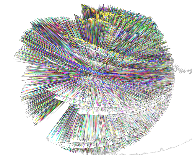
Figure 2. Emotional Layers
Internal Psycho-physiological States and External Facial Expressions
Elena Lyakso, Olga Frolova, and Yuri Matveev’s “Facial Expression: Psychophysiological Study” (Ch. 14) uses FaceReader (v. 8) to study natural interactions between mother-child, child and adults, and other combinations, including in vulnerable populations such as “children with autism spectrum disorders and children with Down syndrome” (p. 266). The various observed emotions are captured as the various research subjects engage in live interactions and pronounce “emotional phrases and words” (p. 269). Here, facial expressions are seen as “the physiological indicator of the human internal state” (p. 273). The co-researchers explore “situations of interactions between mothers and preschool typically developing (TD) children, children with autism spectrum disorders (ASD) and Down syndrome (DS); between orphans and the adult experimenter, children and their peers” in natural conditions (p. 273). The software program labels the emotion and the duration of that emotion in time automatically. This enables researchers to observe down to tenths of a second “the speech behavior strategies of mothers of TD children, children with ASD and children with DS” (p. 276).
They describe some of their findings:
It was found that adults displayed the neural state (78.2% of the time—women and 77.9%--men) and happy (43.7%--women and 25.2%--men) better than other states…The difficulties in manifesting the states of fear (11.2%--women; 0%--men), sadness (9.2%--women; 7.3%--men) were revealed for all adult participants. The text corresponding to the emotion of anger caused in men a better manifestation of the corresponding emotion (15.1%) than in women (5.1%). Men did not show a state of fear (the anger was manifested instead of fear—5.2%). (Lyakso, Frolova, & Matveev, 2021, p. 274)
The co-researchers looking at the emotions expressed and what that might indicate of interrelationships between the parent and child. It is unclear how generalizable this can be given the particular experimental setup. The authors extend some of the assertions:
According to the experts’ answers, mothers of children with DS were more often dissatisfied with their children vs. mothers of children with ASD and TD. Mothers of children with DS smiled less vs. mothers of TD children and children with ASD…In the process of interaction with the mother, children with DS more often were dissatisfied than TD children and children with ASD were. Children with ASD smiled less vs. TD and DS children. (Lyakso, Frolova, & Matveev, 2021, p. 277)
More discussion of the relevance of the work and their application to, perhaps, the care of children and other dimensions, would be helpful.
Effective Facial Expression Synthesis with GAN Architecture
Karthik R., Nandana B., Mayuri Patil, Chandreyee Basu, and Vijayarajan R.’s “Performance Analysis of GAN Architecture for Effective Facial Expression Synthesis” (Ch. 15) highlights the centrality of human nonverbal communication, with facial expressions an important aspect. This team suggests that there are perhaps some universals of facial expression and meaning, such as that “raised eyebrows in combination with an open mouth are associated with surprise, whereas a smiling face is generally interpreted as happy” (p. 290). If artificial intelligence systems should respond to people’s emotions, automated emotion recognition would be important in real time, so interactions with robots and avatars feel natural. Optimally, such a system would work cross-culturally. This work uses four benchmark datasets related to facial expression and emotions: Karolinska Directed Emotional Faces, Taiwanese Facial Expression Image Database, Radboud Faces Database, and Amsterdam Interdisciplinary Centre for Emotion database.
This team uses a Generative Adversarial Network (GAN) approach in order to create synthetic images that may be used as negative examples (distractors that might fool the discriminator or classifier). [Certainly, it is asserted that distractors help make a classifier more robust.] They elaborate:
Sample images were generated by the GAN model during the training phase. Initially, the model was trained for 20,000 iterations instead of 200,000. When the model was tested with test images belonging to the RaFD dataset, the quality of images generated was found to be almost state-of-the-art…However, the model was tested with real time data, and the results obtained were not satisfactory…the expressions generated were found to be visibly distorted rather than convincing or realistic. For this purpose, the model was re-trained with a customized dataset that comprised images of individuals of diverse ethnicities, and with images taken under a wide variety of lighting conditions. (R., B., Patil, Basu, & R., 2021, pp. 303-304)
The various ANNs were run with different architectures, in the Google Colaboratory in the cloud. The model was “trained using Adamax optimizer with hinge loss produced convincing expressions, but at the cost of image quality” (R., B., Patil, Basu, & R., 2021, p. 306). “The test output for the model trained with Stochastic Gradient Descent and hinge loss…produced better images than most other models, while the generated expressions were somewhat subtle” (p. 308).
Object Identification with DCNNs in Constrained and Unconstrained Contexts
Amira Ahmad Al-Sharkawy, Gehan A. Bahgat, Elsayed E. Hemayed, and Samia Abdel-Razik Mashali’s “Deep Convolutional Neural Network for Object Classification: Under Constrained and Unconstrained Environments” (Ch. 16) engages an important idea of “constraints” and “non-constraints” in the environment in terms of the imagesets. Constrained environments mean that there may be less noise in the imageset (from noisy backgrounds, from competing depicted objects, from occlusions, from difficult illumination, from object rotation, and others); unconstrained environments may mean that there is more noise. Unconstrained image data may mean “real-world photos; faces with natural expressions, uncertain shooting angle, in (an) unconstrained environment where there are occlusion and blurs” (p. 333).
If imagesets are to inform work going forward, the challenge of “dataset biasing” (based on image selection) is important to address, so that various leanings of the sets may be accounted for and perhaps made neutral. Computational methods may be applied to resample imagesets to assess for bias. An interesting assumption is that the visual world itself is “unbiased” and that given that imagesets are subsets of the available visuals that they are necessarily biased. There are newer strategies at curating future imagesets or potentially adding augmentations to current ones, to promote improved balance against bias.
The co-researchers write:
Visual cortex models appeared as a solution for bridging the gap between the performance of the human vision and the computational models. Cortical models are bio-inspired systems based on the available neuroscience research to imitate the human visual performance. Neuroscience experiments provide sufficient information to understand how the visual cortex works. Many frameworks appeared as a result of advances and cooperation between several fields like brain science, cognitive science, and computer vision. (Al-Sharkawy, Bahgat, Hemayed, and Mashali, 2021, p. 318)
Deep convolutional neural networks (DCNN) have been found to be superior over prior classical techniques for object classification (Al-Sharkawy, Bahgat, Hemayed, and Mashali, 2021, p. 318). They outperform hand-crafted feature extractors. It is important to have invariance to “shift, scale and distortion,” which means that the classifier can still identify the object from various angles, sizes, and in various contexts (p. 319). Perspective and angle can be highly distortive, as can various lighting. Various deep learning approaches can automatically learn the features without supervision or other inputs beyond the imageset. Advances over the years, especially from 2010 to 2017, have been notable for the precipitous drop in error rates in image classification given newer and new approaches: classical, AlexNet, ZFNet, GoogleNet, ResNet, Trimps-Sushen, and SENet, and others (p. 320).
The co-authors describe the DCNN architecture’s core as the convolutional layer that mimics the simple cells in the visual cortex. The role of the convolutional layer is to “apply filters, known as kernels or receptive fields, to the input and produce feature maps (FMs) that is (sic) also called activation map. Each filter operates on a small spatial dimension of the output of the previous layer to capture the local features. The size of the filter depends on the application of DCNN, but it affects the power consumption, latency and accuracy (Hochreiter, 1998, as cited in Al-Sharkawy, Bahgat, Hemayed, and Mashali, 2021, p. 321). DCNNs do have different architectures. Some are even designed to run on mobile networks. The researchers point to ImageNet Large Scale Visual Recognition Challenge (ILSVRC) competitions as important spaces to bring out innovations.
One challenge in tuning various processes is to avoid overfitting the model to the images in the training set, or else the approach will not generalize well beyond the training imagesets. There are various well known imagesets: NORB, Caltech-256, CIFAR-100, LabelMe, Pascal VOC2012, SUN, Tiny Images, ImageNet, and others. There are dedicated imagesets for particular disciplines and domains, such as the food industry. Each vary in terms of the numbers of images, numbers of categories, numbers of images per category, image resolution (in pixels), sources, and whether the environmental conditions are constrained or unconstrained (Al-Sharkawy, Bahgat, Hemayed, and Mashali, 2021, p. 329). Known weaknesses of DCNNs are “computation time and overfitting problem” (p. 329). DCNNs are known to take comparatively long periods of time to train on target image data because of the “large number of the network parameters in the range of millions that needs (sic) to be optimize and performs (sic) more than 1 Billion (sic) high precision operations (Luan et al, 2018, as cited in Al-Sharkawy, Bahgat, Hemayed, and Mashali, 2021, p. 330).
In some cases, data augmentations potentially help with the discernment work in the classifier modeling. Sometimes, datasets may be too small to have full dimensionality for coverage of the topic. It is beneficial to have a variety of images with levels of difficulty and viewpoints and “intra-class variability” and occlusion (Ponce et al., 2006, as cited in Al-Sharkawy, Bahgat, Hemayed, and Mashali, 2021, p. 334), to better train the deep learning.
Conclusion
Figure 3. Rose Stencil
Alex Noel Joseph Raj, Vijayalakshmi G.V. Mahesh, and Ruban Nersisson’s Deep Learning-Based Image Analysis Under Constrained and Unconstrained Environments (2021) provides an engaging look at how some teams around the world apply various ANNs to image analysis for practical applications, many with clear benefits for humanity, some with some questionable potentials. These examples do generally show mainstream applications and not edge cases. Many of the technologies harnessed were first conceptualized decades ago and only recently came to full fruition with working machine vision and pre-processing and classification algorithms.
About the Author
Shalin Hai-Jew works as an instructional designer / researcher at Kansas State University. Her email is shalin@ksu.edu.
| Previous page on path | Cover, page 15 of 21 | Next page on path |
Discussion of "Book review: Image analysis and classification through image pre-processing and deep learning ANNs"
Add your voice to this discussion.
Checking your signed in status ...