Running a "Deep Learning" Artificial Neural Network in RapidMiner Studio
By Shalin Hai-Jew, Kansas State University
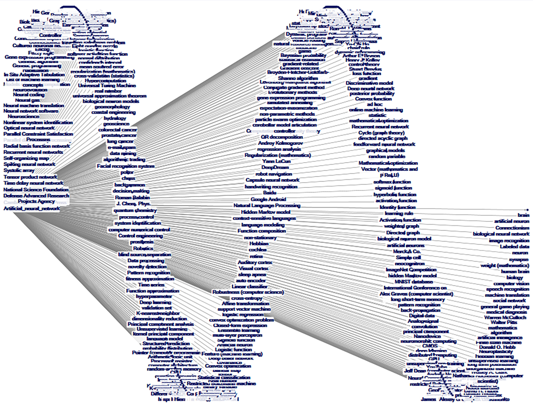
Figure 1. “Artificial_neural_network” Article-Article Network on Wikipedia (1 deg.) (in a horizontal sine wave, with the text scaled-down for readability and less overlap)
The human brain is a complex organ, with some 100 billion neurons, which process signals (chemical and electronic). A single neuron may be connected to some 10,000 other neurons. It is thought that the interconnectivity between the neurons enable various types of sensory and informational processing and that particular pathways are reinforced through experience, exposure, and practice. The respective neural networks are thought to achieve specific functions, when activated, and multiple interconnected ones comprise larger brain networks. This concept of a neural network originates from theorizing in the late 1800s from psychiatrists and early psychologists.
A simplified version of this dimension of the human brain is what informs an artificial neural network (ANN), a type of connectionist system. In this artificial network, there are neurons (or nodes), and they send signals to other neurons in the network. The function of an ANN may be to achieve common objectives of machine learning, including classification, fraud detection, prediction, and other types of analyses for human awareness and decision making. (Simple models of biological neurons are referred to as “perceptrons.” Sometimes, ANNs are referred to as “multi-layer perceptrons.”)
Based on this basic approach, many types of ANNs have been created. A simple one is depicted in Figure 2. The “neurons” are represented by the round nodes, and the “synaptic signals” are represented by the lines (paths for the synaptic signaling). Basically, variables as columnar data is fed into the ANN, and based on observed features, the artificial neural network will reduce the data to particular outcomes. The data is in a basic spreadsheet and / or general dataframe structure, with variables in the column headers, row data as examples, and the information cells as numeric values (including for dummy and for categorical values). There has to be a target variable that will be predicted. The data is run through a number of neurons over a number of different layers (to process different aspects of the data), with subsequent layers dependent on activations in the prior ones. The algorithm enables a “backward propagation” over the respective neurons to make them more appropriately perceptive for the problem at hand (the essential functionality of that particular neural network for the requisite problem-solving).
Figure 2. An Artificial Neural Network (Simple Visual)
The “machine learning” of this setup is in the defining of the proper weights and biases to set for when the various neurons will activate and how the neurons interrelate for the optimal and most accurate output (classification or prediction). The idea is that there are ways to optimize data processing for particular dedicated functions, and these may inform automated and non-automated decision making. One challenge, however, is that creating such models requires a large amount of accurate data. On the other hand, once a model is created, it can be used to process future unlabeled data from similar datasets and can apply accurate predictive labels.
These ANN systems are informed (trained) by the data, whether the data is labeled (for supervised machine learning) or unlabeled (for unsupervised machine learning). Various numbers of hidden layers may be deployed to increase the efficiency of the particular neural network. The balance is between processing time and complexity and the accuracy of the output. The “cost” (square of the error rate) of a particular model is calculated based on the ideal correct labeling of a dataset as compared to what was actually achieved.
Part of the allure of this approach is in the mystery of the hidden layers and how those function and how a computer “thinks” about particular challenges. Another part is the usefulness of this approach in image recognition, with a number recognition dataset as the classic dataset example for this method.
Some additional terms may be helpful. An “iteration” involves a certain number of passes (one full forward and one full backward one, which are considered components of one pass, not two). An “epoch” involves a forward and a backward pass over all of the training examples (in the particular batch). A “batch size” refers to the number of training examples in one forward and backward pass. A full batch contains the entire training set, and a mini-batch refers to the number of training examples in one forward/backward pass.
This article will show the running of the neural network feature in RapidMiner Studio, using a well-known open-source dataset. The run will be done using mostly default settings (which is okay for an early experience but with more experimentation and knowledgeable adjustments in future iterations). A cross-validation will also be run to look at the efficacy of the particular ANN with the labeled data. While the software tool has a fair amount of context-sensitive help and documentation, this article will take a very light approach. Some result data visualizations will be shared. [A limited version RapidMiner Studio is available for free for those in academia for projects which are non-commercial and unfunded through their RapidMiner Educational License Program at https://rapidminer.com/educational-program/].
Running an Artificial Neural Network on RapidMiner Studio
To set up a basic neural network, open RapidMiner. Start a blank New Process. Retrieve the full Titanic dataset. In the Operators, go to the Predictive Models folder, and go to Neural Nets. (Four are available: Deep Learning, Neural Net, AutoMLP, and Perceptron.) In the Deep Learning neural net, select the target attribute value to “Survived”. Click the blue Start arrow at the top left to run. The documentation for this method reads:
Deep Learning is based on a multi-layer feed-forward artificial neural network that is trained with stochastic gradient descent using back-propagation. The network can contain a large number of hidden layers consisting of neurons with tanh, rectifier and maxout activation functions. Advanced features such as adaptive learning rate, rate annealing, momentum training, dropout and L1 or L2 regularization enable high predictive accuracy. Each compute node trains a copy of the global model parameters on its local data with multi-threading (asynchronously), and contributes periodically to the global model via model averaging across the network.
The operator starts a 1-node local H2O cluster and runs the algorithm on it. Although it uses one node, the execution is parallel. You can set the level of parallelism by changing the Settings/Preferences/General/Number of threads setting. By default it uses the recommended number of threads for the system. Only one instance of the cluster is started and it remains running until you close RapidMiner Studio. (RapidMiner Studio 8.2.001)
This software then offers up a range of visualizations. Figure 3 shows some self-organizing maps, originated from three different topographic data compression methods, from the full Titanic dataset. The top two images use the “Landscape,” and the third uses “Fire and Ice” for the applied colors.
Figure 3. Three Self-Organizing Maps of the Titanic Survival Data (with Three Different Drawing Methods)
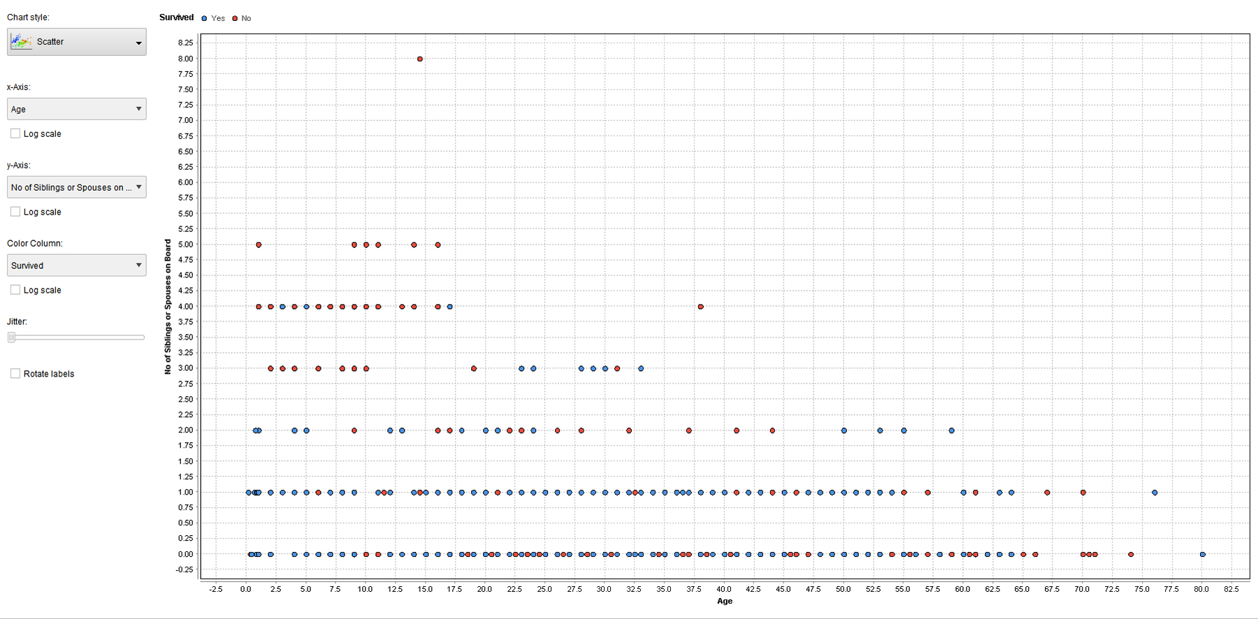
Figure 4 shows the findings in a scattergraph.
Figure 4. Scatter Graph of “Age” and “Numbers of Siblings” in the Labeled Titanic Dataset (processed using an ANN)
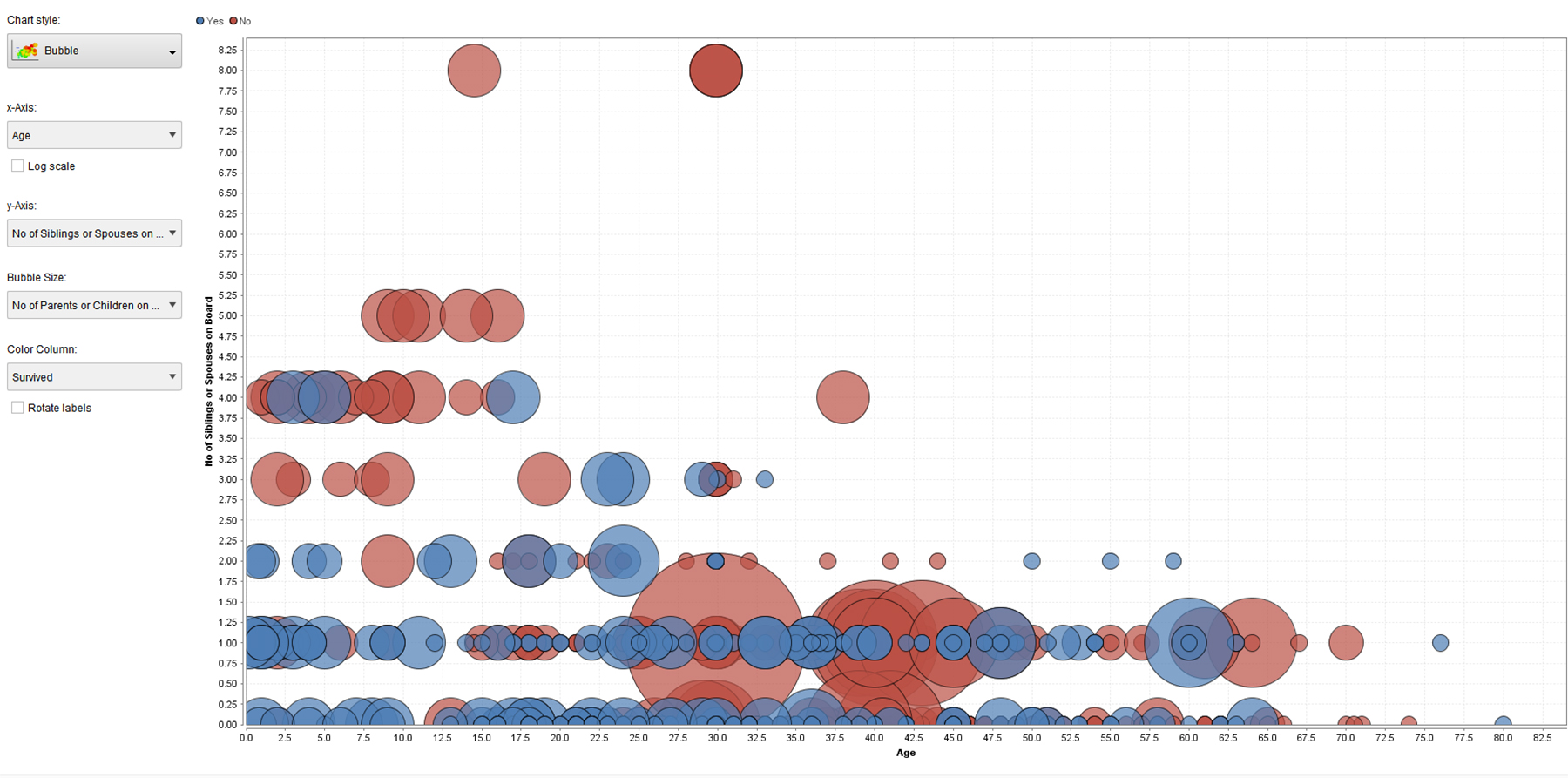
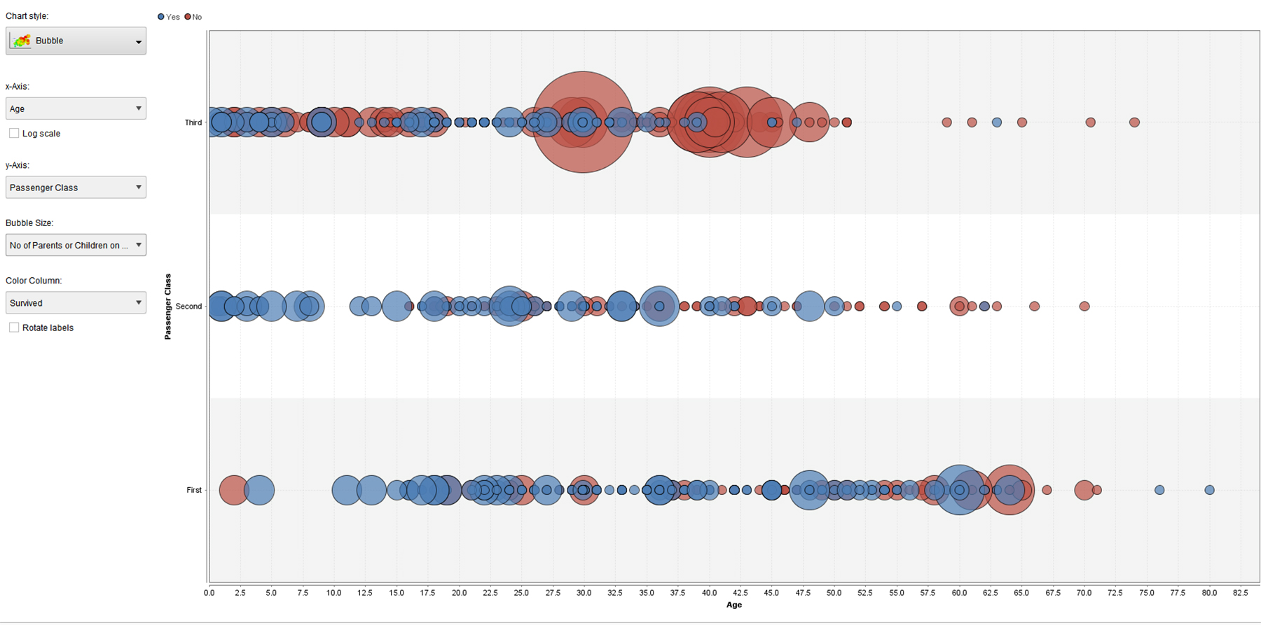
Figures 5, 6, and 7 are all bubble graphs, with variations of variables on the x and y axes and / or different variables portrayed. Note that the blue bubbles are for survivors, and the red ones are for non-survivors. All three enable insights in terms of data patterns (from the data).
Figure 5. Bubble Visualization of “Age” and “Numbers of Siblings” in the Labeled Titanic Dataset (processed using an ANN)
Figure 6. Bubble Visualization of “Age” and “Passenger Class” in the Labeled Titanic Dataset (processed using an ANN)
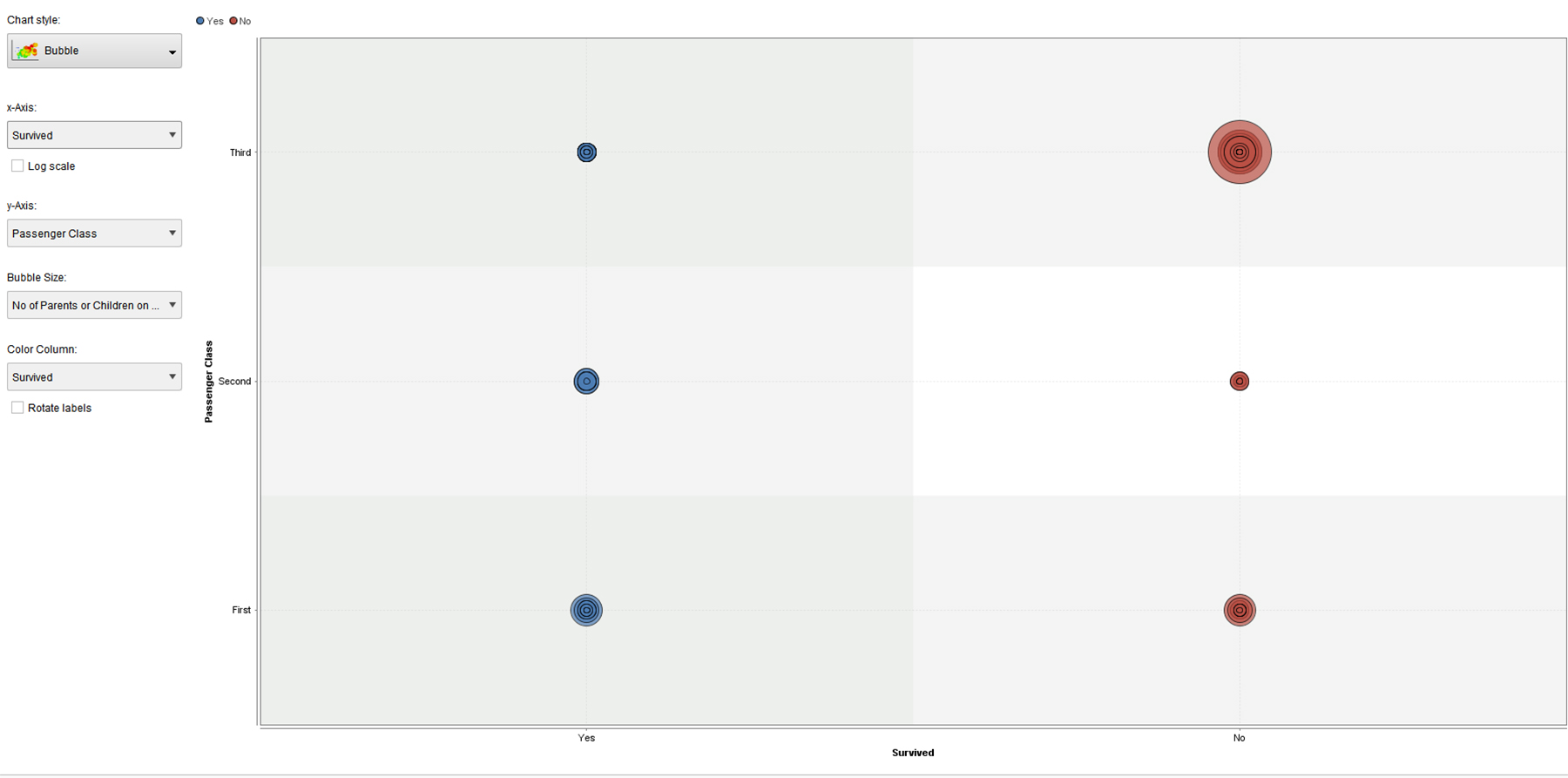
Figure 7. Bubble Visualization of “Survival” and “Passenger Class” Patterns in the Labeled Titanic Dataset (processed using an ANN)
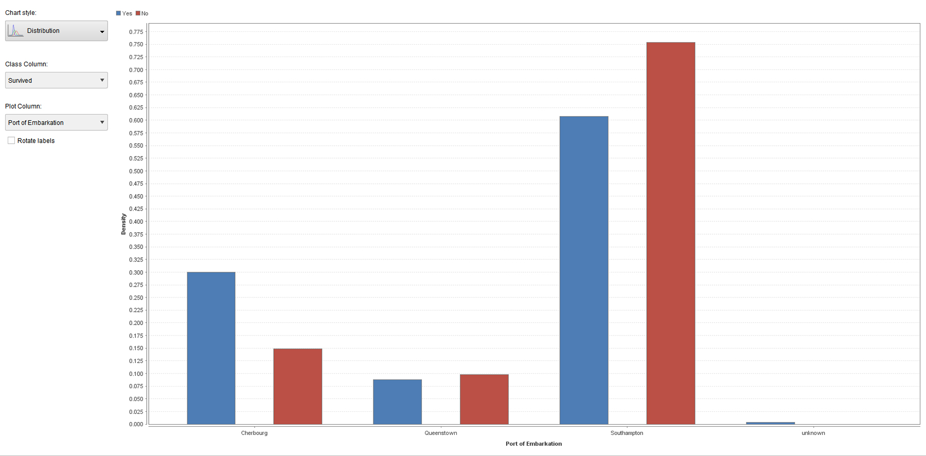
Figure 8 shows the various ports of embarkation (Cherbourg, Queenstown, Southampton, and Unknown) and the survival and nonsurvival. This approach shows a light locational angle to the data.
Figure 8. “Port of Embarkation” and “Survival” in the Labeled Titanic Dataset (processed using an ANN)
Figure 9 shows a scatter matrix summary for a data overview. The “jitter” was set to high to make for larger data points (not to add noise to the data because there really is only a binary with survival/nonsurvival).
Figure 9. Scatter Matrix of the Labeled Titanic Dataset for a Quick Glance at Possible Relational Patterns
The next section shows how the model can be tested for validation (accuracy).
Cross-validation for Model Accuracy
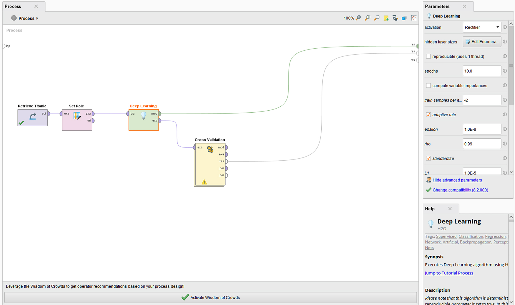
The set up here involves the addition of the cross validation to the sequence. (Figure 10)
Figure 10. A Basic Setup for a Deep Learning ANN in RapidMiner Studio
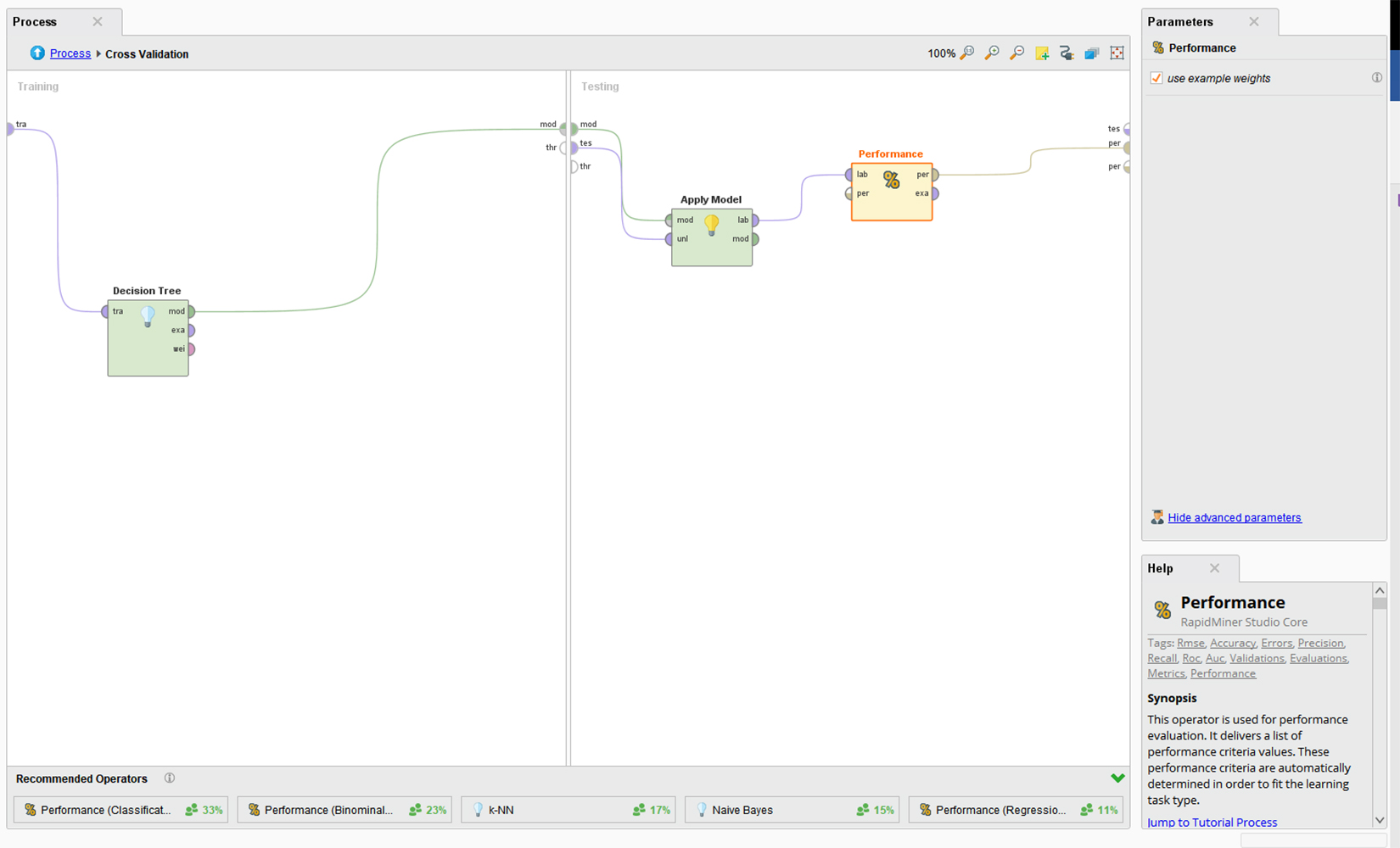
To achieve the cross-validation testing, go to Validation, and select the Cross-Validation. Within the Cross-Validation, set this up with a decision tree informed by the training data in the window to the left, and apply the model to test its performance in the testing window to the right. (This test has 10 folds or iterations as a default setting.) (Figure 11) The software tool has robust help, so follow those directions if there are indicators of missing connections.
Figure 11. A Basic Cross-Validation Setup for the ANN in RapidMiner Studio
Once this all looks good, click the blue Start arrow. There is a built-in tester that offers direct suggestions to fix particular parts of the sequencing.
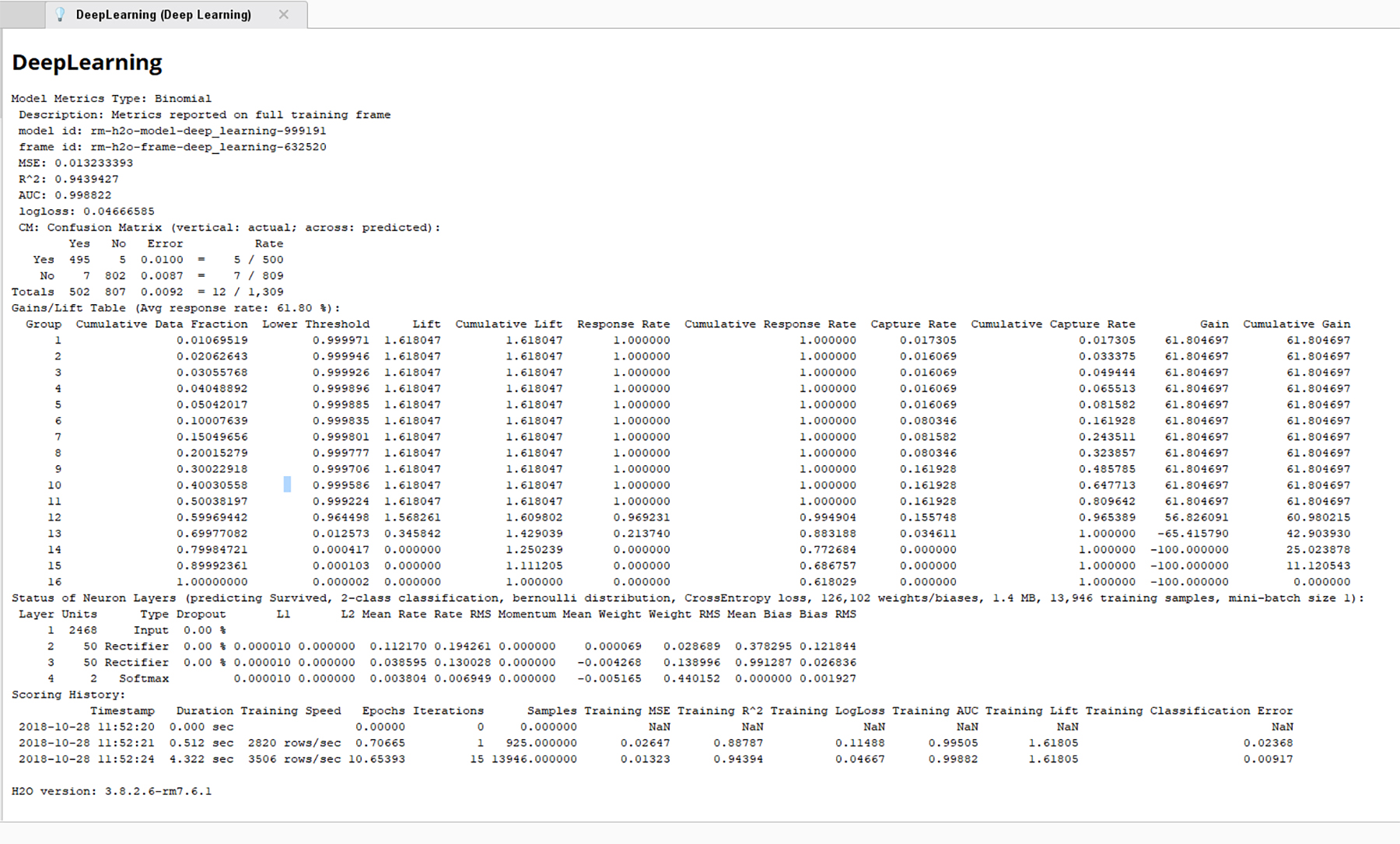
The resulting confusion matrix and report show very low error rates. (Figure 12)
Figure 12. An Error Rate of about 1% (Accuracy Rate of 99%) for the ANN Analysis of the Labeled Titanic Dataset
This is a basic walk-through showing the usage of RapidMiner Studio for setting up and running an artificial neural network. There are a variety of different types of algorithms that run neural networks. Some enable non-forgetting of prior learned patterns, for example. Particular neural network approaches may be more effective for modeling some types of data than others.
For more, Michael Nielsen has a highly recommended free e-book “Neural Networks and Deep Learning” available at http://neuralnetworksanddeeplearning.com/.
3Blue1Brown offers a 4-video neural network series on their channel. The series is available here, and one sample follows below.
Conclusion
Artificial neural networks have been practically applied in a number of contexts to support human awareness and choice making. Applying this method using a very accessible software tool can provide some powerful insights in our respective local work.
About the Author
Shalin Hai-Jew works as an instructional designer at Kansas State University. Her email is shalin@k-state.edu.
She has no direct tie with the makers of RapidMiner Studio.
| Previous page on path | Cover, page 17 of 22 | Next page on path |
Discussion of "Running a 'Deep Learning' Artificial Neural Network in RapidMiner Studio"
Add your voice to this discussion.
Checking your signed in status ...