By Shalin Hai-Jew, Kansas State University
To see how an exploratory factor analysis might work with real-world data, anonymous IT satisfaction survey data from 2014 was used for this light walk-through. The survey instrument itself was a revised inherited open-source survey.
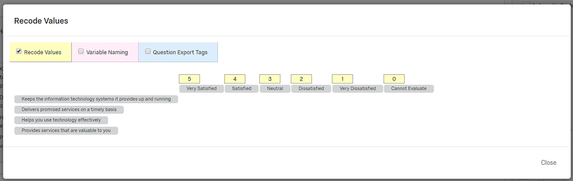
First, before data is used, it has to be downloaded accurately. One step was to recode the Likert-like scores with descending point values instead of ascending point values (Figure 1).
Downloading Data in the Proper Format
Figure 1: Recoding Values from the Survey
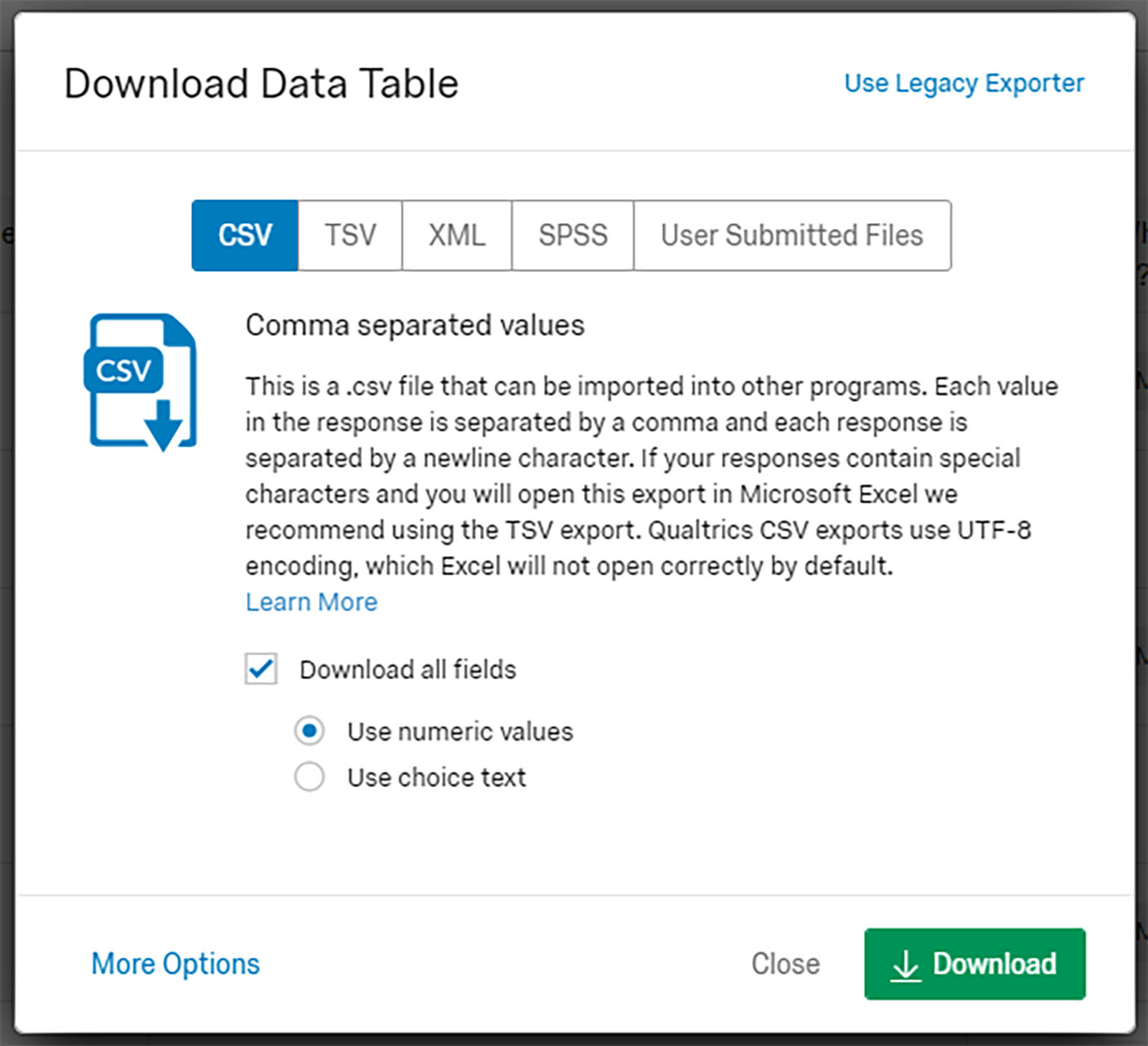
When the data was downloaded, the numerical values were selected—so that the variables (items) could be compared (to see if there were co-associations). (Figure 2)
Figure 2: Downloading the Data Table with Numeric Values
The basic data structure of the extracted information was to have variables in the columns, and the row data were the cases.
The survey itself was exported, so that when the factor analysis was done, the questions and prompts related to the respective variables could be read directly (Figure 3), and text labels could be applied to the extracted factors (components or dimensions). (What should also have been done was a renumbering of each of the questions, so that everything would be in order. Surveys do not come together in perfect order in chronological time, so the renumbering would have brought increased clarity.)
Figure 3: Exporting the Survey to Word
Ensuring Data Meets Requirements for Factor Analysis
There are some data requirements before factor analyses may be run on the data effectively.
Sufficiency of dataset and “some multicollinearity”. Because exploratory factor analysis is a multivariate statistical analysis approach, there have to be a sufficient number of variables that have some similarities among themselves to enable correlations (co-relating). In this survey, there were some 50 usable items for the analysis and 413 responses (but fewer fully completed cases).
The dataset has to have numeric data for the variables. This means that any string (text) data has to be recoded to numeric data or omitted. (In this case, some open-ended questions were omitted as were some complex multi-response questions.)
There have to be a sufficient number of cases (with complete response data per case or per respondent or per row) to enable the identification of factors, in a statistically significant way.
Prior to the factor analysis, some tests were run on the data for
“multi-collinearity.” Some level of multicollinearity is desirable because if variables are unrelated (totally orthogonal), they are not likely to cluster around some related factors. If they are too collinear, then the results might be muddy, with extracted factors being hard to define.
A simple test sometimes used to linearly test multicollinearity is sometimes done (albeit with switching out different variables to be the dependent variable). For this process:
Open IBM's SPSS.
Open a new dataset (wait while it generates a preview).
Work through the Text Import Wizard (for the .csv file). Clarify how the variables are arranged, where the variable names are located (usually in Row 1), the symbol used for decimals, how the cases are arrayed (by rows), the delimiter identification (comma), how dates are represented in the dataset, and so on. Sometimes, it takes several go-arounds to get the underlying data in shape (in Excel first) before it may be opened into SPSS (Statistical Package for Social Sciences).
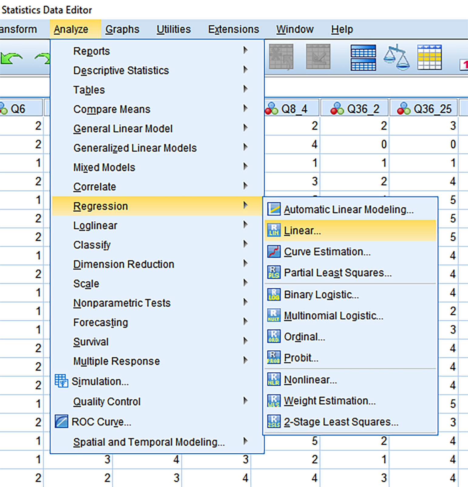
Go to the Analyze tab in the menu. Select Regression -> Linear (Figure 4).
Figure 4: Analyze -> Regression -> Linear
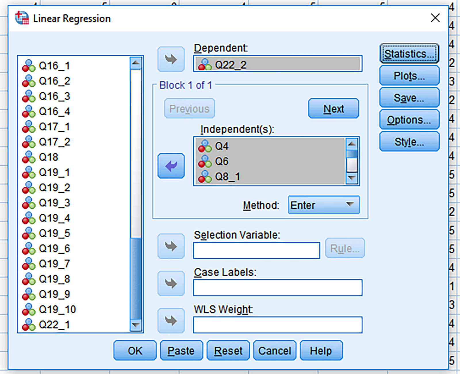
Pick one variable to be the Dependent Variable (DV), and then load the other variables in the Independent Variables (IV) block (Figure 5).
Figure 5: Variables in the Linear Regression
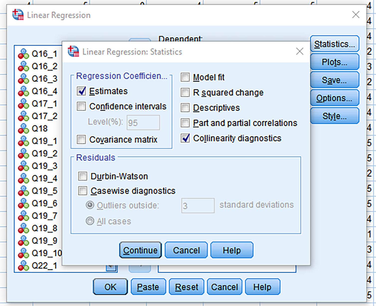
In the Statistics area, select the “Collinearity diagnostics” box (Figure 6).
Figure 6: Selection for Collinearity Diagnostics
In the Coefficients table, check the column for collinearity statistics. “Tolerance” refers to how variable one independent variable is that is not explained by the other independent variables. The desirable cutoff for tolerance is said to be between 0.10 to 0.25 as the minimum tolerance (
"Tolerance," 2017). For the “VIF” or Variance Inflation Factor, this index “measures how much the variance (the square of the estimate’s standard deviation) of an estimated regression coefficient is increased because of collinearity” or correlation with other predictor variables (
"Variance Inflation Factor," 2017). The highest level of VIF that is acceptable is 10 (
“Variance Inflation Factor,” 2017) A few variables go over that in this dataset…from the one run linear regression (Table 1). (As noted earlier, this should be run multiple times with different variables in the DV position.)
Table 1: Coefficients Table
On the whole, though, this data works. There is some degree of multicollinearity but not excessive amounts. There are sufficient cases, and there are sufficient variables (items).
Running the Exploratory Factor Analysis in SPSS
Again, the assumptions of an “exploratory” factor analysis is that the researcher does not have initial hypotheses about factors in the data. There are no applied theories or frameworks or other a priori assumptions. There are no hypotheses being tested with the factor analysis. (If there were a priori assumptions, then the type of factor analysis being conducted would be a “confirmatory” factor analysis. The process would be the same, but the analytical approaches would be different.) Figure 7 shows how to start a factor analysis.
Figure 7: Analyze -> Dimension Reduction -> Factor
In the related windows, it is important to include all variables in the factor analysis. In the section for the Correlation Matrix, the Kaiser-Meyer-Olkin (KMO) test should be run in order to see how well the dataset is set up for the extraction of factors, and the related Bartlett’s test of sphericity (which tests for homogeneity of variances and how normal an underlying frequency distribution is for a set of data). Extract a correlation matrix. Extract a scree plot. Set the factor extraction based on factors with eigenvalues greater than 1 (instead of selecting a desired number of factors, at least not initially). Go with the default maximum iterations for convergence at the default of 25. The factor analysis rotation may be set at Promax with a Kappa of 4. Select any other desirable matrices. Exclude cases listwise (if there is incomplete information in a case, then it is left off altogether from the factor analysis.) Select the coefficient display format to be sorted by size (from the biggest factors to the smallest), and suppress small coefficients at 0.30 to start. (The default in SPSS is set to 0.10.)
Resulting Factor Analysis
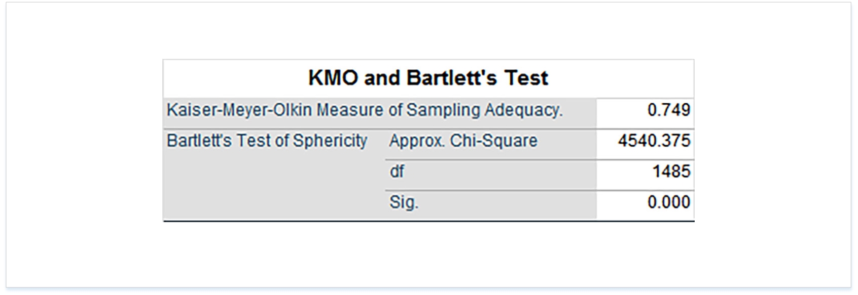
As noted earlier, the KMO indicates how likely it would be for this dataset to enable some factors (sub-groups) to be extracted. A KMO score would ideally be 0.80 or higher, and in this case, rounded up, this dataset just makes. The statistical significance for Bartlett’s Test is sufficient (Table 2).
Table 2: KMO and Bartlett’s Test of Sphericity
A study of “communalities” shows how much an item correlates with all other items, and Table 3 shows some fairly high correlations, which suggests some communal coherence among the variables.
Communalities
|
|
Initial
|
Extraction
|
Q4
|
1.000
|
0.743
|
Q6
|
1.000
|
0.533
|
Q8_1
|
1.000
|
0.704
|
Q8_2
|
1.000
|
0.772
|
Q8_3
|
1.000
|
0.780
|
Q8_4
|
1.000
|
0.684
|
Q36_2
|
1.000
|
0.701
|
Q36_25
|
1.000
|
0.670
|
Q36_3
|
1.000
|
0.663
|
Q36_29
|
1.000
|
0.749
|
Q36_6
|
1.000
|
0.696
|
Q36_4
|
1.000
|
0.766
|
Q36_18
|
1.000
|
0.713
|
Q36_26
|
1.000
|
0.671
|
Q36_15
|
1.000
|
0.706
|
Q36_9
|
1.000
|
0.688
|
Q36_30
|
1.000
|
0.750
|
Q36_7
|
1.000
|
0.716
|
Q36_5
|
1.000
|
0.734
|
Q36_8
|
1.000
|
0.608
|
Q36_10
|
1.000
|
0.566
|
Q36_16
|
1.000
|
0.690
|
Q36_12
|
1.000
|
0.668
|
Q36_19
|
1.000
|
0.725
|
Q36_27
|
1.000
|
0.784
|
Q36_11
|
1.000
|
0.614
|
Q36_31
|
1.000
|
0.711
|
Q10_1
|
1.000
|
0.918
|
Q10_2
|
1.000
|
0.903
|
Q10_3
|
1.000
|
0.825
|
Q12_1
|
1.000
|
0.732
|
Q12_2
|
1.000
|
0.639
|
Q12_3
|
1.000
|
0.860
|
Q12_4
|
1.000
|
0.817
|
Q14_1
|
1.000
|
0.824
|
Q14_2
|
1.000
|
0.779
|
Q14_3
|
1.000
|
0.576
|
Q16_1
|
1.000
|
0.895
|
Q16_2
|
1.000
|
0.861
|
Q16_3
|
1.000
|
0.819
|
Q16_4
|
1.000
|
0.895
|
Q17_1
|
1.000
|
0.708
|
Q17_2
|
1.000
|
0.744
|
Q18
|
1.000
|
0.746
|
Q19_1
|
1.000
|
0.724
|
Q19_2
|
1.000
|
0.914
|
Q19_3
|
1.000
|
0.668
|
Q19_4
|
1.000
|
0.757
|
Q19_5
|
1.000
|
0.812
|
Q19_6
|
1.000
|
0.785
|
Q19_7
|
1.000
|
0.724
|
Q19_8
|
1.000
|
0.802
|
Q19_9
|
1.000
|
0.649
|
Q19_10
|
1.000
|
0.715
|
Q22_1
|
1.000
|
0.679
|
Q22_2
|
1.000
|
0.793
|
Extraction Method: Principal Component Analysis.
|
Table 3: Communalities
Figure 8 shows a scree plot. This line graph shows the loadings of extracted factors above an eigenvalue of 1 (where the red line is). This visualization shows the 14 factors that had fairly significant loading by variables in this particular dataset.
Figure 8 : Scree Plot
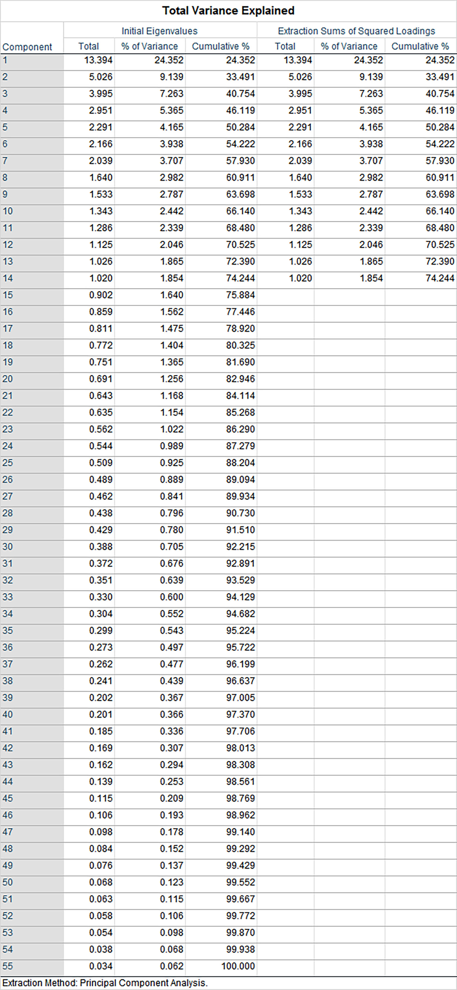
Table 4, the “Total Variance Explained,” shows that this factor analysis can explain a cumulative 73.872% of the variance in this dataset.
Table 4: Total Variance Explained
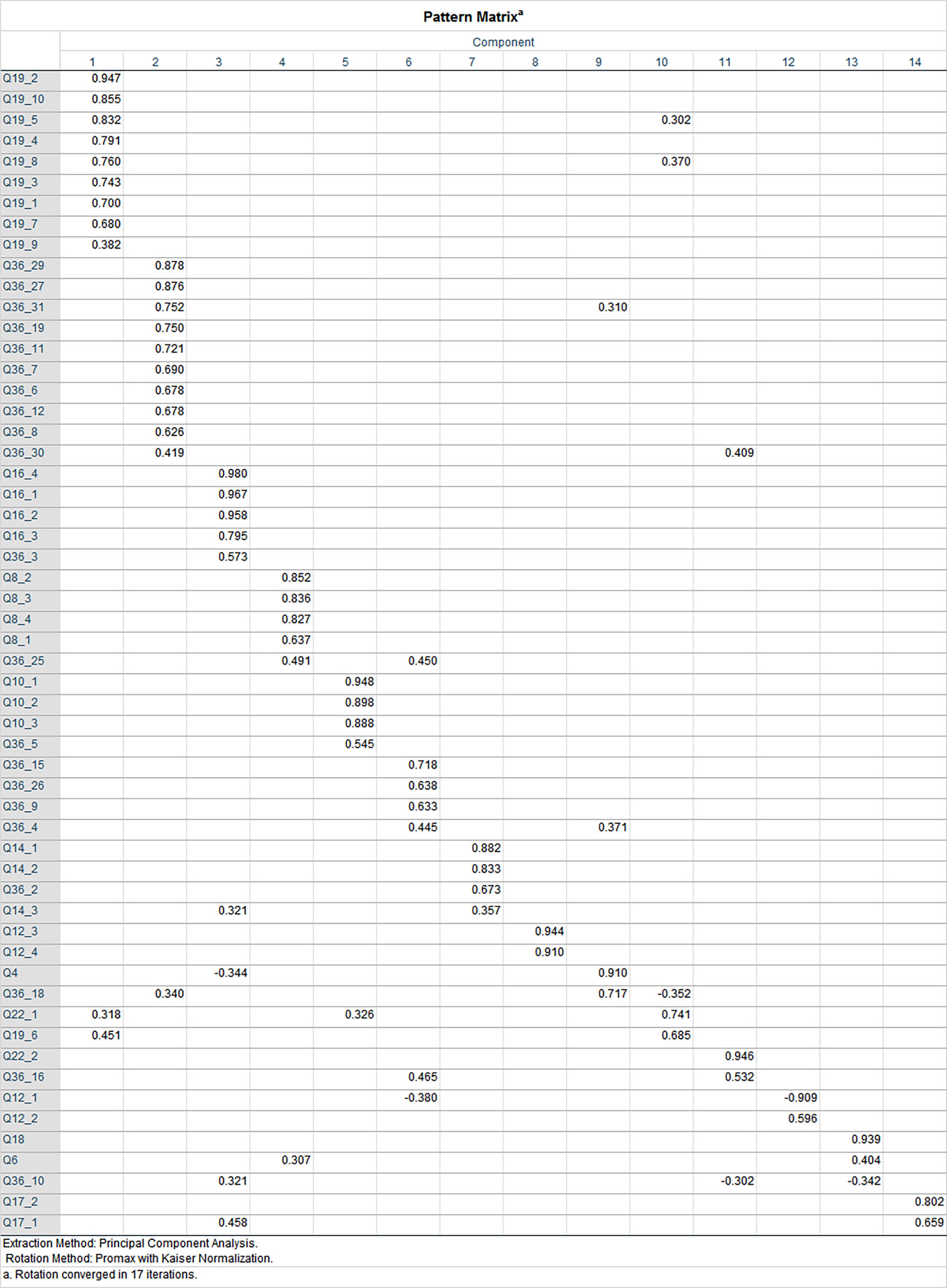
In Table 5, the Pattern Matrix, the fourteen “common” factors may be seen in the column headers in descending order. The coefficients in the pattern matrix show how the variables in the left column load to the respective factors. Cross-loadings, when variables load to two factors (with less than a .2 difference), are usually addressed by eliminating the variables sequentially and seeing if that may be done without ending up with a failure to converge in 25 rotations. The variables with problematic crossloadings are the following: Q36_30, Q36_25, Q36_4, Q14_3, Q36_18, Q22_1, Q36_16, Q6, and Q36_10.
If the variables cannot be removed without causing problems in the rotation, then another approach is to raise the threshold for inclusion of loading. In this case, the loading coefficient was set to 0.4, which resulted in a much cleaner pattern matrix, with only three variables cross-loading. Increased cumulative variance was explained (74.244%), with 14 factors.
Table 5: Pattern Matrix
The next step, once a pattern matrix has been cleaned up, is to label the variables with human-readable text for sense-making. (To see the second pattern matrix, please
click here.) In this case, one has to return to the survey to read the related questions and prompts for the loading items…in order to label them. (Also, a component correlation matrix can be run to see how the factors correlate with each other.)
So the variables that loaded to the respective factors were as follows:
Factor 1: Q19_2, Q19_10, Q19_5, Q19_4, Q19_8, Q19_3, Q19_1, and Q19_7
Factor 2: Q36_29, Q36_27, Q36_31, Q36_19, Q36_11, Q36_7, Q36_6, Q36_12, Q36_8, and Q36_30
Factor 3: Q16_4, Q16_1, Q16_2, Q16_3, and Q36_3
Factor 4: Q8_2, Q8_3, Q8_4, Q8_1, and Q36_25 (albeit with co-loading)
Factor 5: Q10_1, Q10_2, Q10_3, and Q36_5
Factor 6: Q36_15, Q36_26, Q36_9, and Q36_4
Factor 7: Q14_1, Q14_2, and Q36_2
Factor 8: Q12_3 and Q12_4
Factor 9: Q4 and Q36_18
Factor 10: Q22_1 and Q19_6
Factor 11: Q22_2 and Q36_16
Factor 12: Q12_1 and Q12_2
Factor 13: Q18 and Q6
Factor 14: Q17_2 and Q17_1
The applied labels to the respective factors were as follows:
1. Network Function and Reliability
2. IT Physical Spaces and Direct Services
3. Telephone Services
4. Tech Services / Follow-through
5. Help Desk Support and Availability
6. User Accounts, CONNECT Services, Survey Tool, Web Services
7. Computer Technologies in Classrooms
8. Mobile Friendly Technologies
9. Gender and ?
10. Availability of Network and Mobile
11. File Storage Location and Network Speed
12. Mobile Friendly Technologies
13. Wifi Availability on Campus
14. Strength of Signal, Availability of Connectivity on Campus
Table 6: Named Factors
Ideally, names for these factors (components or dimensions) should be much more parsimonious.
Assessing the Reliability of the Factors
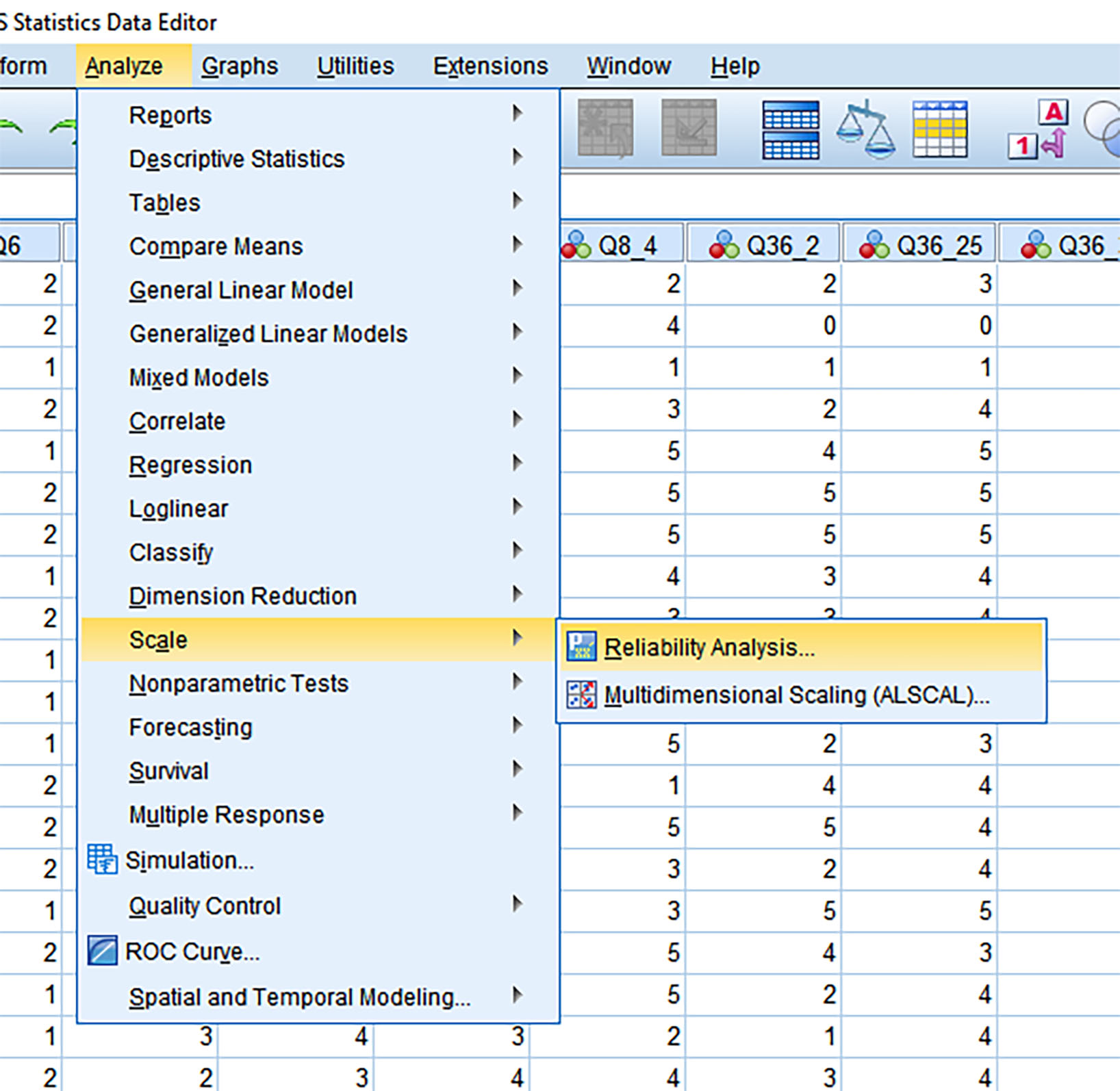
Finally, some researchers test the reliability of the respective factors by bundling the respective variables underlying each factor and running a reliability analysis on them (to see how coherently the respective factors are describing a particular construct). For this, Cronbach’s alpha is captured as a representation of reliability (Figure 9).
Figure 9: Analyze -> Scale -> Reliability Analysis
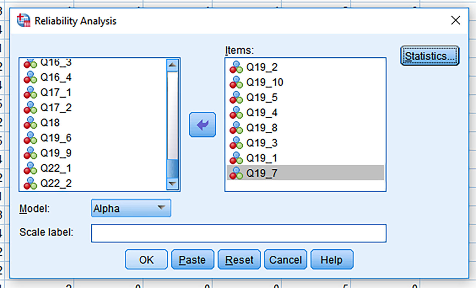
Figure 10 shows the selection of the variables that loaded to Factor 1.
Figure 10: Variables for Factor 1 Selected
The reliability analyses result in a Cronbach’s alpha score. The general cutoffs suggest that .6 and over is acceptable, .7 to .9 is good, and .9 is excellent… in terms of how well the variables represent a coherent construct (or factor). If the numbers are lower than .6, the reliability of the elements representing the factor construct is unreliable…and may not be indicating a coherent or valid component.
Factor Numbers (in descending order)
|
Variables / Items
|
Topic / Applied Name to the Factors
|
Cronbach’s Alpha (for reliability)
|
1
|
Q19_2, Q19_10, Q19_5, Q19_4, Q19_8, Q19_3, Q19_1, and Q19_7
(8 items / variables)
|
Network Function and Reliability
|
0.93
[182 (44.1%) cases valid cases, 231 (55.9%) excluded (based on listwise deletion)]
|
2
|
Q36_29, Q36_27, Q36_31, Q36_19, Q36_11, Q36_7, Q36_6, Q36_12, Q36_8, and Q36_30
(10 items / variables)
|
IT Physical Spaces and Direct Services
|
0.905
[312 (75.5%) cases valid cases, 101 (24.5%) excluded]
|
3
|
Q16_4, Q16_1, Q16_2, Q16_3, and Q36_3
(5 items / variables)
|
Telephone Services
|
.927
[304 (73.6%) cases valid, 109 (26.4%) excluded]
|
4
|
Q8_2, Q8_3, Q8_4, Q8_1, and Q36_25 (albeit with co-loading)
(5 items / variables)
|
Tech Services / Follow-through
|
.819
[326 (78.9%) cases valid, 87 (21.1%) excluded]
|
5
|
Q10_1, Q10_2, Q10_3, and Q36_5
(4 items / variables)
|
Help Desk Support and Availability
|
.914
[314 (76%) cases valid, 99 (24%) excluded]
|
6
|
Q36_15, Q36_26, Q36_9, and Q36_4
(4 items / variables)
|
User Accounts, CONNECT Services, Survey Tool, Web Services
|
.720
[325 (78.7%) cases valid, 88 (21.3%) excluded]
|
7
|
Q14_1, Q14_2, and Q36_2
(3 items / variables)
|
Computer Technologies in Classrooms
|
.779
[310 (75.1%) cases valid, 103 (24.9%) excluded]
|
8
|
Q12_3 and Q12_4
(2 items / variables)
|
Mobile Friendly Technologies
|
.826
[225 (54.5% cases valid, 188 (45.5%) cases excluded]
|
9
|
Q4, Q36_18
(2 items / variables)
|
Gender and ?
|
.113
[319 (77.2%) cases valid, 94 (22.8%) excluded]
|
10
|
Q22_1 and Q19_6
(2 items / variables)
|
Availability of Network and Mobile
|
.669
[298 (72.2%) valid, 115 cases (27.8%) excluded]
|
11
|
Q22_2 and Q36_16
(2 items / variables)
|
File Storage Location and Network Speed
|
.713
[305 (73.8%) cases valid, 108 (26.2%) excluded]
|
12
|
Q12_1 and Q12_2
(2 items / variables)
|
Mobile Friendly Technologies
|
-.254
“The value is negative due to a negative average covariance among items. This violates reliability model assumptions. You may want to check item codings.”
[279 (67.6%) cases valid, 134 (32.4%) excluded]
|
13
|
Q18 and Q6
(2 items / variables)
|
Wifi Availability on Campus
|
.035
[295 (71.4%) cases valid, 118 (28.6%) excluded]
|
14
|
Q17_2 and Q17_1
(2 items / variables)
|
Strength of Signal, Availability of Connectivity on Campus
|
.619
[305 (73.8%) cases valid, 108 (26.2%) excluded]
|
Table 7: Measuring the Reliability of the Respective Factors by Variables with Cronbach’s Alpha
Table 7 communicates the descending order of reliability of the factors. Factors 9, 12, and 13 were not considered reliable.
Conclusion
Ideally, the exploratory factor analysis would be explicated in depth in a research context. The underlying survey instrument would be available for analysis. The data would be fully explored in other ways beyond the EFA. How respondents interacted with the survey could be mentioned, and light item analysis may be done.
In this case, the data was fairly dated. It looks like the original online survey had been revised after the initial offering, so the downloaded data referred to responses to questions no longer available on the Qualtrics site. (The variable "Gender and ?" points to the missing block of variables.) This data was used as a walk-through, though, and the outputs still make sense even with the known limits to the data.
About the Author
Shalin Hai-Jew is an instructional designer at Kansas State University. Her email is shalin@k-state.edu.
Discussion of "An Exploratory Factor Analysis of IT Satisfaction Survey Data (from 2014)"
Add your voice to this discussion.
Checking your signed in status ...