Applying “Survival Analysis” to Instructional Design Project Data
By Shalin Hai-Jew, Kansas State University
Traditionally, “survival analysis” is a statistical representation of the speed of human decline, under varying health and other conditions. This representation is based on empirically observed data, and from this data, a regression curve is extracted--from which data generalizations may be made (about similar populations in similar contexts). This data can reveal times of heightened risk, and in that sense, it could indicate possible critical times for extended surveillance and possible interventions.
Simply, at the beginning of the research (Time Zero), there is a population of individuals who are fully present. Over time, members fail to survive and drop out. At any particular time, there is a survival rate or S(t) which is known as “survival at time t”. Survival is conceptualized in part as a factor of time, and it is a factor of “hazard” or the risk of non-survival. The higher the hazard rate, the lower the survival rate; the converse is also true: the lower the hazard rate, the higher the survival one (these rates have a negative correlation).
As noted earlier, these observations may be applied to other similar populations for deeper understandings. They may be applied to different populations to see if there are differences in survival rates: for example, one group may serve as a control, and another may be the group that receives some intervention to prolong survival. The comparisons made are between population curves to observe differences. With sufficiently large population sets, there may be an underlying assumption of a normal survival distribution (a Gaussian distribution), but there is no such assumption for smaller population sets which may be convenient data sets and which are not particularly random (and therefore not representative of a full normal distribution and not broadly generalizable). With sufficiently large populations, though, z-scores may be extrapolated, and statistical significance of findings may be applied. Also, in terms of data, the longer the time period studied, the more data that may be included.
Figure 1: Sample Survival Function Plot
What a simple survival analysis graph shows, simply, is the time-to-event of death in a non-increasing line graph. (The reason why the line is not described as decreasing is because there are times of plateaus or non-loss of a member from the original population.) Another way to think about this is as a measure of attrition from a particular population over time. Time may be measured as a continuous set of values or as discrete ones. In this example, time is treated as discrete and measured in monthly units (more granularly measured time is not necessary in this example).
The hazard function is seen to be non-decreasing and will trend up with cumulative hazard over time. The “hazard” concept is something like “risk” based on empirical observations of events. In a simple survival analysis model, hazard is a constant over time. In real world contexts and more sensitive models, the hazard function changes over time and may increase or decrease. (A classic example of a hazard curve is the "bathtub curve," which is intuitive and worth a look.)
"Censoring"
So why don’t statisticians just use a normal linear regression to capture such changes over time? The thinking is that survival analyses include "censored" data in the time-series analysis. Data censoring refers to the dropout rate of persons in a survival analysis—due to the ending of the research period or a lack of follow-through of research participants with researchers; such normal random censoring is beyond the control of researchers. Including censored data in a survival analysis helps mitigate "survivorship bias" in statistical analysis--or overweighting the effects of the data points that "survive" the research period and come to researcher attention but not counting or acknowledging the data that drops out of the study or is not considered or seen by the researcher. (Mitigating "survivorship bias" requires researchers to ask themselves to consider what data they're not seeing and not including when they design their research.)
In this case, it helps to conceptualize a timeline with the past to the left and the future to the right. Here, “left censoring” refers to the lack of knowledge of researchers of what has happened with participants before they were included in a study, and “right censoring” refers to the completion of the research before the individuals experience the event (non-survival in some cases). After the research is complete, researchers will not be following up with the remaining or surviving participants and so do not know what happens to them (although they may be able to infer what will happen given the captured data from others in that particular cohort). Research observations are censored when the data about their survival time is undetermined or incomplete. This censoring information, even though it is a data limitation, provides richer real-world information for analysis.
In the same way that all the population is alive at Time 0, there is a point in the future when the entire population is no longer present. It is in the in-between time that there is research interest. For example, there may be periods of intensification of non-survival ("critical phases")…or long periods of survival and non-events…or spates of censoring due to in-environment events or other factors.
There are a variety of variations to these basics. Besides censoring, research projects may have individuals enter at different times in what is known as staggered entry. There are statistical methods to enable study of multiple events…in a survival analysis, and other insights. For this work, a very basic survival analysis will be explored but with real-world and original data.
Basic Data Elements of a Survival Analysis
To operationalize a survival analysis, researchers have to be able to define a few important elements. So what basic data is needed in a survival analysis? A researcher needs the following:
• a particular population (or phenomenon or object) to study,
• defined units of time (at what level of granularity), and
• what an “event” (non-survival, in the classic survival analysis sense) looks like (objectively).
Time is the independent variable, and time-to-event is the random (outcome) variable. There may be variables (called "covariates" in survival analysis) that affect survival outcomes: positively or negatively, and to varying degrees. Some of these covariates may contribute to hazard, which decreases the time-to-event (or "non-survival"). Some covariates such as health interventions may lower hazard and increase the time-to-event (or "non-survival").
Now that the basic elements have been explained, it is important to conceptualize “survival analysis” in other ways. For example, it may be thought of as time-to-event.
Various Applications of “Survival Analyses”
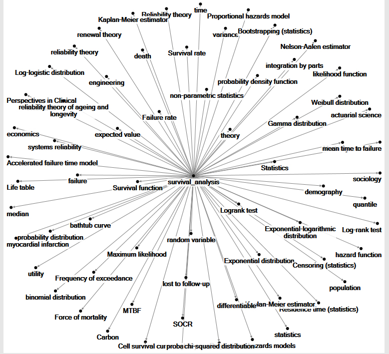
A “survival analysis” may be applied to many more contexts than people passing on from a population. Other forms of survival analysis are also known as “time-to-event” analysis, event history analysis, reliability analysis, and duration analysis, and variations on this method are applied in engineering, economics, sociology, and other fields. To have a sense of the breadth of “survival analysis,” it may help to view the article network around the Wikipedia article about this in Figure 2.
Figure 2: A “Survival_Analysis” Article Network on Wikipedia (1 deg.)
See if you can identify the “survival analysis” or “time-to-event” aspects of the following questions:
- In political science, what is the time-to-event for a nation-state to reach full collapse?
- In sales and marketing, what is the time-to-event for a groomed potential customer to actually purchase the particular merchandise?
- In sociology, what is the time-to-event for social movements to emerge into a powerful entity?
- In public health, what is the hazard rate of a newborn in a particular population to acquire a particular disease?
- In education, what is the survival rate of learners in the STEM (science, technology, engineering, and math) pipeline (from pre-K all the way through graduate school and beyond)?
- Or how long do learners stay in a particular online learning degree program? Or the college or university before they either graduate or drop out?
- In education, what is the time-to-event for a freshman to earn a baccalaureate degree?
- In a help desk ticketing system, how long do tickets remain open before they are closed, and how many are never closed (censored)?
The general examples above show that the “event” does not have to equal the demise of the subject. The event may be what many may consider a net positive.
There are various types of data structures underlying survival analyses, different computations that may be applied to the data, and different software programs that may be used for such analyses. This particular article will use IBM’s SPSS.
Survival Analyses in Education
Survival analysis, even in its simple form, can be applied to education. Essentially, any phenomenon that has a start-and-stop time element can be depicted in a survival analysis. This is not to say that these are run in a discovery or exploratory method outside the context of some research questions, research design, and hypothesizing.
To see how this might work, survival analysis was run on instructional design (ID) projects from 2010 – 2016. The original set of objects are the projects, and the “events” are completion with bills sent to the principal investigators (PIs) / faculty owners of the instructional design projects. The start date is artificial since there are data from prior (to 2006), but the billing for prior projects were purchases of half-a-year of instructional designer time...for multiple projects...and those are somewhat beyond the focus of this example (pre-bought time guarantees the project unless the instructional designer fails spectacularly in follow-through on the work).
Censored projects are those for which no paid work was done—so in these cases, there were early discussions of work and initial recording of hours, but nothing ultimately came of the work for various reasons. One way to conceptualize censoring is of somewhat incomplete work, something that has not been taken to its full actualization. (Left out entirely from this research are the thousands of consultations and works for which no pay was ever expected because the projects did not rise to the design and development level of funded work. Also left out are the many in-depth multi-year projects which occurred as part of the higher education ecosystem…but for which no funds were directly moved between university units. And finally, there is the grant-chasing work done on various projects. In many cases, no funds are directly acquired. In other cases, grant funds are attained but are distributed more locally to the respective colleges and departments, but no payments were made to the instructional designer.) While the underlying data here are real, the specifics have been removed because these are not important to the method and would not contribute to deeper understandings in this context.
It is thought that such “time-to-event” studies may improve the management of instructional design projects, so that these move from the stages of light talk to actual work and actual completion of paid work. The paying for work often is correctly conflated with the use of the learning objects. Unpaid projects are often not political priorities and garner much less administrative protection over time. While there are many ways to complete instructional design work successfully and to help the university attain a “win,” those projects will not be discussed here.
Hazarding Educated Guesses (“Hypothesizing”)
Understanding which ID projects thrive may shed light on the “hazards” that make a project sufficiently successful (based on the prior terms). As such, this set may be split into two: those that make to "event" and those which "censor" out. Then the respective characteristics of the respective instructional design projects in each grouping may be compared. Another built-in way to break apart the groups into categories is by length of project. Yet another is to cluster projects by high-cost vs. low-cost (with various bounds for each). These categories may be defined already with the given data. The topics of the respective projects may be analyzed, too, based on the redacted data (which is known to the researcher and may be coded in future work).
Beyond those features mentioned earlier, it would help to identify other attribute features of the respective instructional design projects. These may include the following variables:
- types of deliverables
- existence of pre-defined designs
- standards for the instructional build
- defined technical platforms
- requirements to use proprietary technical platforms
- size of development team
- complexity of the targeted learner population
- whether there is need to collaborate with other institutions, and others
Once the respective features are defined and the individual projects are duly coded, it will be possible to analyze survival analysis of the respective sub-clusters of instructional design projects for time-pattern differences. For survival analyses involving multivariate data, researchers go to the Cox Regression survival analysis (which is one of four survival analysis types in SPSS).
From the above, there will be a list of "askable questions" based on data queries and data visualizations.
- For example, of the set of ID projects which achieve to “event,” how does that set differ from those that end up “censored”? Is it possible to anticipate what sort of ID project may be in one category or the other?
- How do types of required project deliverables affect survival, "event," and censoring?
- Are pre-defined designs a net positive or a net negative in terms of project attainment of "event" / completion?
- Do collaborations with off-campus entities mean projects take longer periods or shorter periods to complete? Or are such off-campus collaborations not a factor?
- and so on...
Real-world debriefing. From experience, projects that are pre-funded with a federal grant tend to proceed to funded work. Those ID projects with required and defined online course or learning objects will generally result in successful instructional design and project completion and payment to the unit. In part, those projects have to meet stringent legal requirements on a number of fronts: intellectual property protections, accessibility, and so on. These also have to survive project assessment by a third-party entity, and these have to show learning gains. Projects that have strong leadership, a line-up of talent, a clear plan, and sufficient resourcing tend to do well and achieve “event” instead of being “censored”.
Censoring does not always occur due to limitations of the project PI. An instructional designer may have to decline a project because the project requirements are not attainable given local skills and local resources. In that case, IDs have to self-censor projects. If PI expectations are too high in terms of what the technologies can achieve, that is another scenario in which self-censoring of projects occurs. Early and clear communications are critical to help identify projects which are a mismatch with ID capabilities and skills (which vary greatly depending on units).
Instructional Design on a University Campus
It may help to describe the instructional design context on this particular university campus. For some years, instructional design was generally provided as a service to all faculty who requested the service. However, as time passed, it became clear that some clients were those who had federal grant dollars who needed intensive builds (whole online courses or learning sequences, sophisticated websites, and other objects). An official university rate card was created to address these types of projects that required more than the complimentary initial 10 hours. While some long-term instructional design projects were created for free—given the political horse trading on campuses—these tend to be outliers…maybe only a half-dozen in a decade of ID work at this institution, at least based on the experiences of one instructional designer.
Billing for such projects requires approvals by the principal investigators (of grants) / faculty members. Some projects extend over a budget year and may require multiple bills. In general bills are finalized at the ends of projects within budget years but occasionally, a few projects may extend over a fiscal year. The average bill for an instructional design project between 2010 – 2016 was $2,488.85, with this average skewed by several projects paying in the five digits. The period of research was seven years (or 84 - 4 = 80 months since this was done at the end of August 2016). The projects were entered in a staggered entry, and the length of project time would be the months of work spent on the project. Twenty-six projects were identified, with a min-max cost range of $400 to $34,000.
On this campus, because of the sparsity of funds, the idea is to get any ID service gratis and move on without any bill if possible, so it’s important for an instructional designer to discuss the rate card and expectations early on.
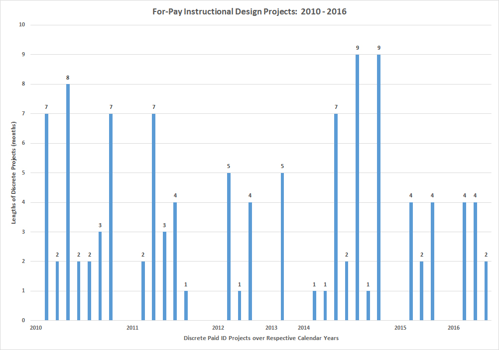
The average length of time from the start of a project to the end is four months. Rarely, talks will start on a project many months before actual start of project because the funding has not come in until then. The start of a project begins with the first contact with the recording of the gratis hours. For many projects, if it seems that the work will only be consultation without full design and development, those hours are only recorded on a work calendar, and no bill is even started. Bills are only started if there is discussion of more extensive paid work. In Figure 3, the various ID projects with bills are listed. That said, there are sometimes periods of drought for paid work on a campus. Also, the years here are calendar years, not fiscal years (which start in July and end at the end of June the next year).
Figure 3: For-Pay Instructional Design Projects: 2010 – 2016
Setting up for the Survival Analysis
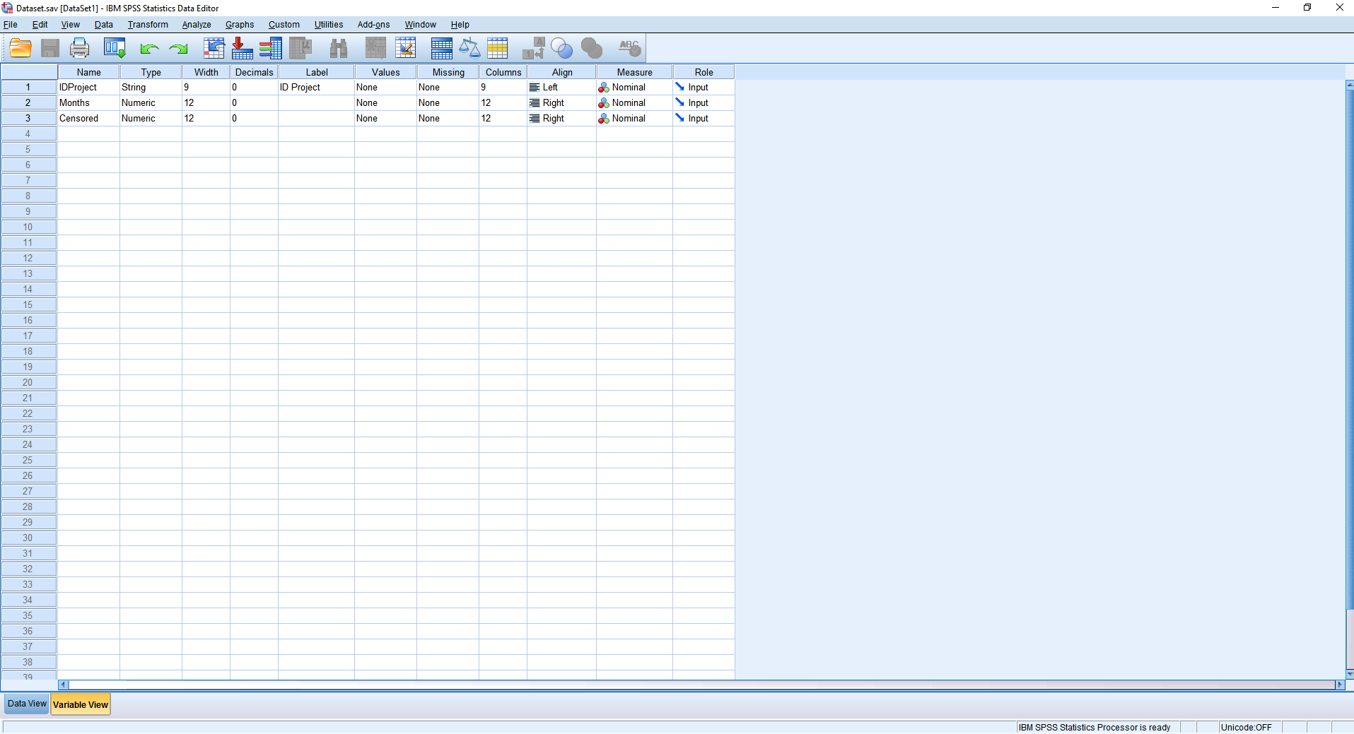
Setting up the data for this survival analysis begins with a review of bill files. From these files, what is captured are the following: the general name of the project, start dates, end dates, and final bill amount (if any). The length of the projects are calculated from the start- and end- dates with the unit time being months. If a project resulted in a bill, that would be labeled a “1” for “event,” and if a project did not result in a bill, that would be labeled a “0” to represent “censored.” This information is represented in three columns:
| ProjectName | UnitTime (or "Spell") | EventorCensored |
|---|
The first column is comprised of string data written in camel case; the second is integer data; the third is a dummy variable represented either with a 1 (event) or a 0 (censored), presence or absence. The resulting table data was run through a survival analysis using the Kaplan-Meier estimate in SPSS. The Kaplan-Meier method originated in 1958 and is known as "the product limit estimator". The ingested data may be viewed in Figure 4.
Figure 4: Instructional Design Survival Analysis Data in SPSS
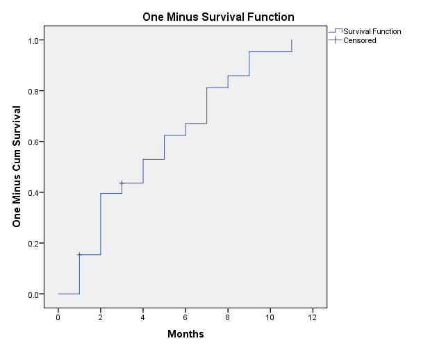
According to the Case Processing Summary, this analysis identified an N = 26, with 23 of these achieving “event” (billed services) (88.5% of the set) and 3 “censored” (non-billed services) (11.5% of the set). The survival table captured 26 time events (Figure 5).
Figure 5: Redacted Survival Analysis Table from the Instructional Design Dataset
By the first month in, 19% of the instructional design projects have reach event. By the end of the second month, 42% of projects have achieved event or been censored, and only 58% survive. By the fifth month, there is only 35% of projects are still in limbo--without either a determination of whether they will be a paid project or will censor out of the study. None of the projects exist in the unbilled or censored categories by the 11th month, so a decision for whether a project will continue as a billed one or not is decided within a calendar year of the start of the project.
The average survival time is 4.613 months, with a standard error of .625, with the 95% confidence interval’s lower and upper bounds at 3.388 to 5.838. The median survival time is 4, with a standard error of 1.089, with a 95% confidence interval at 1.865 and the upper at 6.135. (The confidence bounds assume an underlying normal curve, which may be an inaccurate assumption. In all likelihood, the underlying distribution is non-normal, given the topic.)
Another way to conceptualize this data is by percentile. At the 25th percentile, a project may take about 7 months (with a standard error of .593). At the 50th percentile, representing half of all projects, these take 4 months (with a standard error of 1.089). On the 75th percentile (third quartile), under which 75% of the projects may be found, these projects take approximately 2 months (with a standard error of .403). All of the quartile values of the K-M estimate are within the ranges and so are defined values). In other words, the majority of projects tend to be fairly short; said another way, rarer projects may be longer.
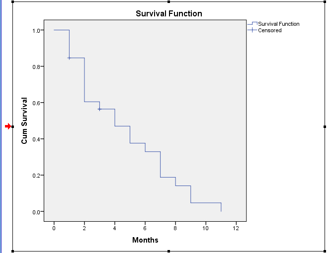
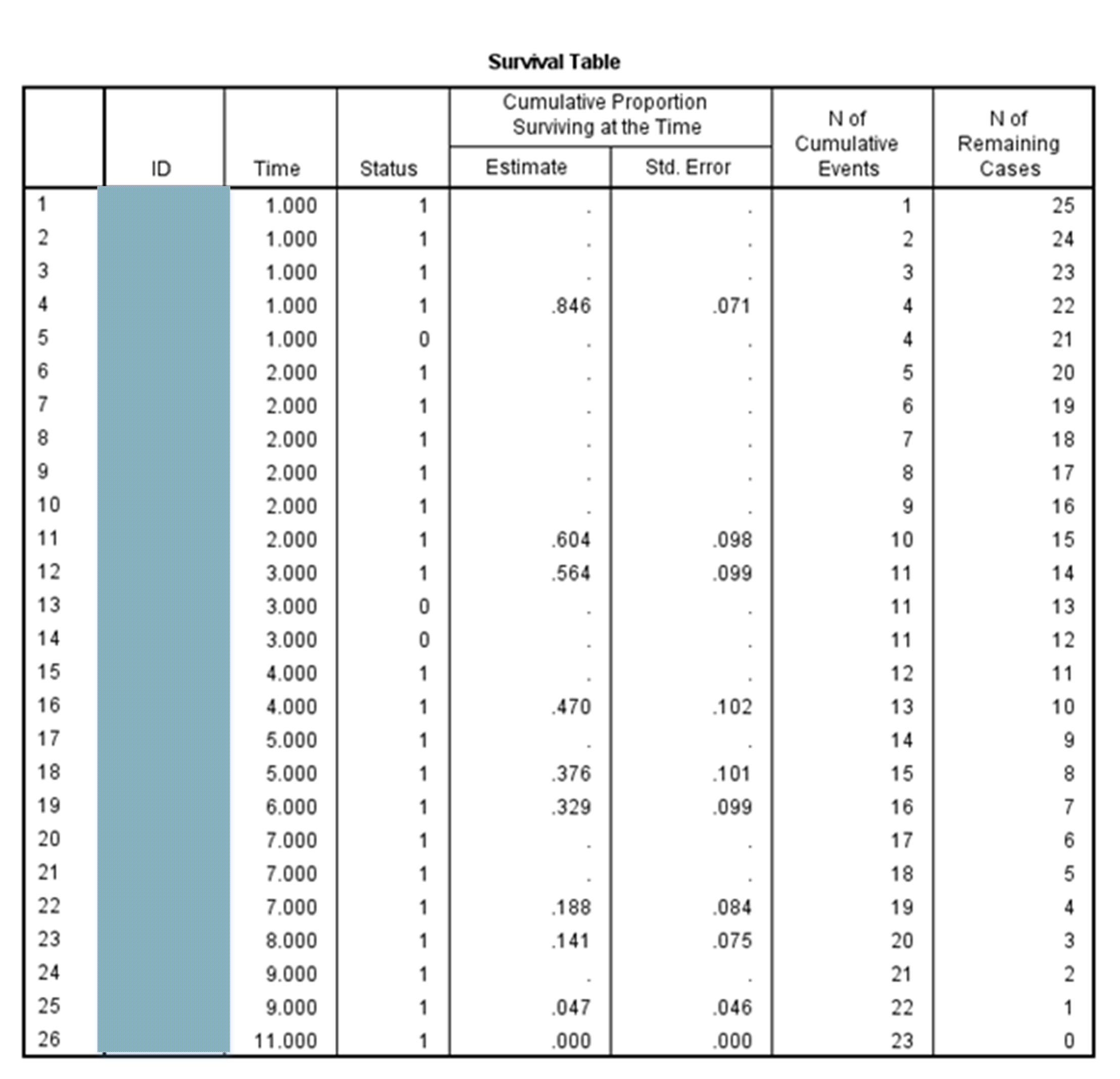
Figure 6 shows the survival function curve for these 26 instructional design projects. Note on the y-axis “CumSurvival” (cumulative survival) that the full set is present at the top left with a score of 1, representing full survival of the full set of ID projects. As time passes (as indicated on the x-axis), the curve changes in a stair-step way. When the line is parallel with the x-axis, that plateau shows that there was no project event occurrence. As the line moves perpendicular to the x-axis, that shows a drop-off of projects over time, which indicates the experience of an ”event” (the paying of the project). The “plus,” if you will, shows a project being censored of leaving the set without payment. Note that the censoring does not result in a change to the curve (whether up or down). This line cannot be called a decreasing line graph because of the moments of plateau where there is no decrease. At the bottom right of the plot, the population of instructional design projects has been dissipated through events or censorship to 0 at around the 11-month mark.
What the linegraph suggests, visually, is that projects that will censor are identified early and end early. In other words, if it is clear that a project will not be funded, it tends not to continue for long periods of time. Also, most projects achieve “event” at fairly regular intervals at one month, two months, and so on. Longer projects past nine months tend to go to nearly a year. So survival of a project is depicted here as a function of time. The S(t) [the “s” of “t”] or survival at time t may be understood from the linegraph. The more time that passes, the more likelihood that a project will result in pay as long as the project hasn’t ended by being censored out.
Figure 6: “Survival Function” Applied to Instructional Design Projects
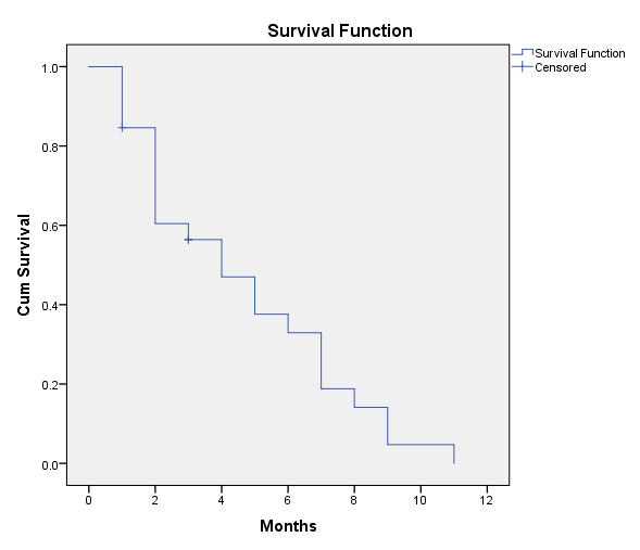
This same data may be visualized as a hazard function. In Figure 8, the line of the graph starts at the bottom left. At (0,0), the origin of the graph, the hazard function is the same for all the instructional design projects. Over time (expressed in the horizontal x-axis), the hazard rate starts to manifest. One sign of that is in month one when the line moves vertically, indicating an event (based on the hazard). And so, it all stair-steps upwards cumulatively. The hazards seem to occur earlier in the lifespan of an instructional design project and actually seems to lessen once Month 9 has been reached.
Figure 7: “Hazard Function” Applied to Instructional Design Projects
In the instructional design context, it helps to know whether a project formalizes into a paying one. It helps to have the hypothesizing around the desirable “hazards” to ensure that a project makes it to successful fruition and mutual benefits for the respective university units involved.
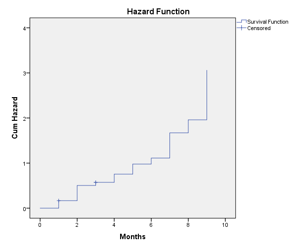
This same data may be plotted in a One Minus Survival Function (Figure 8). This shows a line that grows over time. At any point in the line, an individual may capture the cumulative incidence rate at that particular point in time. The “one minus” part works because both survival and hazard are plotted on a range from 0 – 1 (for normalized probability data). One minus survival [1-S] equals the cumulative hazard rate and also equals the rising incidence of non-survival (event) as seen in time (or time segments).
Figure 8: Accumulating Incidence of ID Projects Achieving Event in the One Minus Survival Function Plot
Debriefing
First, it is important to mention that a naive interpretive approach will be unhelpful. Some naive assertions from these "survival analysis" findings may go as follows:
- If I stretch out the time of a project, I will achieve completion and payday.
- If a project censors early on, it will not be recoverable and may never achieve "event."
And based on the early interpretations, some naive assertions may continue:
- A PI with access to federal funds will always be a paying client (most are super frugal, which is good for the institution of higher education overall, but which guarantees a small payday, if any).
What are some more sophisticated insights from these graphs? These may suggest which types of projects to target. A cursory analysis of the underlying data shows that the projects that are generally funded tend to be from the health sciences and agriculture because those are priorities for federal grant funding agencies. Also, federal compliance trainings sometimes result in some project payment (but would more likely result in gratis work because these benefit the campus broadly and are politically justifiable in the work unit). It would be possible to identify PIs who tend to spearhead successful projects. It would be possible to identify which projects may end up in a lot of healthy work and a fair payout based on an analysis of variables which often lead to project success.
It may be possible to separate out the various projects (such as by topical groups) in order to run log-rank survival analyses against these groups to see if there are fundamental differences between these groups. In these visualizations, there are two or more survival lines running through the graph which enable comparison.
Clearly, it is helpful to understand the underlying context in order to better interpret the data. It is important to know the data itself fairly well to know how to accurately interpret the findings.
In this example, limited but real-world data were used to run a survival analysis in SPSS to surface some basic insights about the “state” of instructional design at one institution of higher education. These are incomplete data, and some data were redacted here. However, this example should give a sense of how a basic survival analysis may work.
Conclusion
"Survival analyses" may be used not only to describe time-to-event data in a descriptive way (to enable hypothesizing and analysis), but they may be used as models to understand other similarly situated data and to even enable predictions of out-of-sample data. These predictions may inform expectations of future events, with varying levels of confidence. Certainly, as new data is available, it is possible to integrate more data to the survival analyses for the prior applications.
A survival analysis is a straightforward statistical analysis approach that can have wide applications in higher education to provide insights about time-based phenomena (pretty much everything). This approach can provide data points and insights for faculty, administrators, staff, and students.
A Data Visualization Addendum
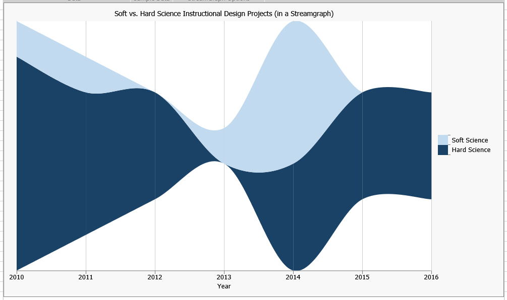
Sometimes, I catch myself saying that I am mostly funded by those in the hard sciences vs. the soft sciences. Since I'd only recently discovered how to make a streamgraph in Excel 2016, I thought I would map out the number of soft vs. the hard science instructional design projects I'd worked per each of the years from 2010 - 2016. It turns out that while I do work more hard science projects, there were some soft sciences ones as well. The differential between the sizes of the projects are highly weighted towards the hard science projects, too, but that's another story.
About the Author
Dr. Shalin Hai-Jew works as an instructional designer at Kansas State University. She may be reached at shalin@k-state.edu.
| Previous page on path | Issue Navigation, page 19 of 25 | Next page on path |
Discussion of "Applying “Survival Analysis” to Instructional Design Project Data"
Add your voice to this discussion.
Checking your signed in status ...