Cluster Analysis
INCOMPLETE DRAFT
In order to use cluster analysis successfully to interpret literary texts, it is important to have a good understanding of how the process works.
Cluster analysis may be formally defined as an unsupervised learning technique for finding “natural” groupings of given instances in unlabeled data. For the purposes of text analysis, a clustering method is a procedure that starts with a group of documents and attempts to organize them into relatively homogeneous groups called “clusters”. Clustering methods differ from classification methods (supervised learning) in that clustering attempts to form these groups entirely from the data, rather than by assigning documents to predefined groups with designated class labels.
Cluster analysis works by counting the frequency of terms occurring in documents and then grouping the documents based on similarities in these frequencies. When we observe that an author or text uses a term or a group of terms more than other authors or other texts do, we are innately using this technique. In making such claims, we rely on our memory, as well as sometimes unstated selection processes. It may be true, for instance, that Text A uses more terms relating to violence than Text B, but in fact, the difference between the two may be proportionally much less than the difference in the frequency of other terms such as “the” and “is” on which we do not traditionally base our interpretation. Cluster analysis leverages the ability of the computer to compare many more terms than is possible (or at least practical) for the human mind. It may therefore reveal patterns that can be missed by traditional forms of reading. Cluster analysis can be very useful for exploring similarities between texts or segments of texts and can also be used as a test for hypotheses you may have about your texts. But it is important to remember that the type of clustering discussed here relies on the frequency of terms, not their semantic qualities. As a result, it can only provide a kind of proxy for meaning. In order to use cluster analysis successfully to interpret literary texts, it is important to have a good understanding of how the process works.
Document Similarity
In traditional literary criticism, concepts like “genre” are frequently used to group texts. There may be some taxonomic criteria for assigning texts to these groups, but recent work in Digital Humanities (Moretti, Jockers, Underwood) have highlighted that such categories can be usefully re-examined using quantitative methods. In cluster analysis, the basis for dividing or assigning documents into clusters is a statistical calculation of their dis(similarity). Similar documents are ones in which there is considerable homogeneity in the frequency with which terms are observed to occur therein. Documents are dissimilar when term frequencies are more heterogeneous.
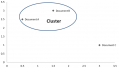
A clearer picture emerges of this definition of similarity if we examine how it is measured. Imagine three documents as points within a coordinate space.
Document A can be imagined to be more similar to Document B than to Document C by using the distance between them as a metric. Simply draw a straight line between the points, and the documents with the shortest line between them are the most similar. When using cluster analysis for the study of texts, we take as our premise the idea that this notion of similarity measured in distance may correlate to a range of historical and stylistic relationships amongst the documents in our corpus.
The graph above represents the end of the process. In order to plot our documents in coordinate space, we must first determine the coordinates. This is done by counting the terms in our documents to produce a document-term matrix. For instance a part of the document-term matrix that produced the graph above might be:
| man | woman | |
|---|---|---|
| Document A | 5 | 4 |
| Document B | 4 | 5 |
| Document C | 1 | 3 |
The list of term counts for each document is called a document vector. Representing the text as a vector of term counts allows us to calculate the distance or dissimilarity between documents. We can easily convert the document-term matrix into a distance or dissimilarity matrix by taking the difference between the term counts for each document vector.
| Man | Document A | Document B | Document C |
| Document A | - | 1 | 4 |
| Document B | 1 | - | 3 |
| Document C | 4 | 3 | - |
The distance from A to B is 1 while the distance from B to C is 3. Documents A and B form a cluster because the distance between them is shorter than between either and Document C.
Notice that the table above reproduces only the portion of the document vectors representing the frequency of the word “man”. Adding the “woman” portion creates considerable difficulties for us if we are trying to represent the data in rows and columns. That is because each term in the document vector represents a separate dimension of that vector. The full text of a document may be represented by a vector with thousands of dimensions. Imagine a spreadsheet with thousands of individual sheets, one for each term in the document, and you get the idea. In order for the human mind to interpret this data, we need to produce a flattening, or dimensionality reduction, of the whole distance matrix. The computer does this by algorithmically going through the distance matrix and adjusting the distance between each document vector on the observed distances between each of the terms. There are, in fact, different algorithms for doing this, and part of a successful use of cluster analysis involves choosing the algorithm best suited for the materials being examined.
Many discussions of this process begin with the notion of feature selection. In text analysis, this equates to determining what features of the text make up the document vector. The procedure for feature selection is essentially the processes of scrubbing, cutting, and tokenization. You may also perform certain normalization measures that modify the term frequencies in order to account for differences in document length. Depending on how you perform these tasks, the results of cluster analysis can be very different. One of the factors that will influence your results is your choice of distance metric.
The distance metric is essentially how you define the difference between your documents. A simple example might be the words cat and can (think of these words as documents composed of vectors of three letters each). A distance metric called edit distance can be defined as the number of changes required to transform cat into can (1). The difference between cat and call would be 2. For longer documents, using an edit distance metric would not make sense, so we need some other way of defining distance. A classic definition of distance between two documents is the Euclidean distance,which is essentially the length of a line between two points in the document vectors (your choice of linkage method determines which points get used for this calculation). The Euclidean distance metric measures the magnitude of the difference between the two document vectors.
Another approach is to measure the similarity of the two vectors. A common method of doing this is to calculate the cosine similarity, which is the angle between the vectors. Cosine similarity is not truly a measure of distance, but it can be converted into a distance measure by subtracting the cosine similarity value (which varies between 0 and 1) from 1.
The difference between Euclidean and non-Euclidean metrics for measuring document distance is largely one of perspective. Euclidean distances tend to measure the distance between documents at some point along the vector where the documents are already quite distinct from one another. In longer documents, this distinction may correlate to a lot of terms which are found in one document but not the other. In the document-term matrix, counts for these terms in the documents where they do not occur are recorded as 0. A distance matrix in which most of the elements are zero is called a sparse matrix. The more dimensions there are in the document vectors, the more likely it is that the distance matrix will be sparse. Measuring Euclidean distance in a sparse matrix can affect the way clustering takes place. We would certainly expect this to be the case if one document was much longer than the other. Using cosine similarity as the basis for measuring distance is one way to address this problem by using the angle between document vectors, which does not change depending on the location of points along the vector. There are a large variety of variants on these basic Euclidean and non-Euclidean approaches to defining the distance metric for clustering. For further discussion, see Choosing a Distance Metric.
Other factors influencing your results will depend on the type of cluster analysis you use.
Types of Cluster Analysis
There are two main approaches to clustering: hierarchical and partitioning. Hierarchical clustering attempts to divide documents into a branching tree of groups and sub-groups, whereas partitioning methods attempt to assign documents to a pre-designated number of clusters. Clustering methods may also be described as exclusive, generate clusters in which no document can belong to more than one cluster, or overlapping, in which documents may belong belong to multiple clusters. Hierarchical methods allow clusters to belong to other clusters, whereas flat methods do not allow for this possibility. Lexos implements two types of cluster analysis: a form of hierarchical clustering called agglomerative hierarchical clustering and a form of flat partitioning called K-Means.
While a full discussion of the many types of cluster analysis is beyond the scope of this work, we may note two other methods that are commonly used in literary text analysis. One such method is topic modeling, which generates clusters of words that appear in close proximity to each other within the corpus. The most popular tool for topic modeling in Mallet, and the Lexos Multicloud tools allows you to generate topic clouds of the resulting clusters from Mallet data. Another type of clustering is often referred to as community detection, where algorithms are used to identify clusters of related nodes in a network. More information about community detection in network data can be found here [needs a link].
Strengths and Limitations of Cluster Analysis
Cluster analysis has been put to good use for a variety of purposes. Some of the most successful work using cluster analysis has been in the area of authorship attribution, detection of collaboration, source study, and translation (REFs). Above all, it can be a useful provocation, helping to focus enquiry on texts or sections of texts that we might otherwise ignore.
It is important to be aware that there is not a decisive body of evidence supporting the superiority of one clustering method over another. Different methods often produce very different results. There is also a fundamental circularity to cluster analysis in that it seeks to discover structure in data by imposing structure on it. While these considerations may urge caution, it is equally important to remember that they have analogues in traditional forms of an analysis.
Regardless of which method is chosen, we should be wary of putting too much stock in any single result. Cluster analysis is most useful when it is repeated many times with slight variations to determine which results are most useful. One of the central concerns will always be the validity of algorithmically produced clusters. In part, this is a question of statistical validity based on the nature of texts used and the particular implementation chosen for clustering. But there is also the more fundamental question of whether similarity as measured by distance metrics corresponds to similarity as apprehended by the human psyche or similarity in terms of the historical circumstances that produced the texts under examination. One of the frequent complaints about cluster analysis is that, in reducing the dimensionality of the documents within the cluster, it occludes access to the content--especially the semantics of the content--responsible for the grouping of documents. Point taken. Treating documents as vectors of term frequencies ignores information, but the success of distance measures on n-dimensional vectors of term counts is clear: cluster analysis continues to support exploration that helps define next steps, for example, new ways of segmenting a set of old texts.
The following sections will be removed to a separate page.
Hierarchical Clustering
Hierarchical cluster analysis is a good first choice when asking new questions about texts. Our experience has shown that this approach is remarkably versatile (REF). Perhaps more than any one individual method, the results from our cluster analyses continue to generate new interesting and focused questions.
Hierarchical clustering does not require you to choose the number of clusters to begin with. The clusters that result from hierarchical clustering are typically visualized with a two-dimensional tree diagram called a dendrogram. This dendrogram can be built by two methods. Divisive hierarchical clustering begins with only one cluster (consisting of all documents) and proceeds to cut it into separate “sub-clusters”, repeating the process until the criterion for dividing them has been exhausted. Agglomerative hierarchical clustering begins with every document as its own cluster and then proceeds to assign these items to “super-clusters” based on some similarity for similarity. Since the resulting tree technically contains clusters at multiple levels, the result of the cluster analysis is obtained by “cutting” the tree at the desired level. Each connected component then forms a cluster for interpretation. One of the challenges for the interpreter is where to cut the tree. For more information about the construction and interpretation of dendrograms, see the video below:
A crucial part of the algorithm is the criterion used for establishing the distance between clusters. Typically, we may select from three possible methods.
- Single linkage
- Complete linkage
- Average linkage
Need to add discussion of Euclidean and other metrics.
In our test cases, we have yet to identify a case where the Euclidean metric with average linkage failed to provide the most meaningful results. However, Lexos allows you to apply a number of algorithms and compare the results. This may be one method of establishing the robustness of a clade.
Considerations:
Hierarchical clustering does not scale well. With many documents the number of computations can be strain on a computer’s processing power. Even when it is possible to produce a dendrogram, the resulting graph, with tens of clades or more, may be impossible to read (and therefore interpret).
- All items are forced into clusters. (isn't this also true here?)d
Another issue is that documents tend to be divided into clusters early during the process, and the algorithm has no method for subsequent undoing of this partitioning.
K-Means Clustering
Partitions a data set into some arbitrary number (k) of clusters, using some criterion. The algorithm has the following steps:
Partition the data into k non-empty subsets.
Create centroids for each cluster. The centroid is the center (mean point) of the cluster. In some implementations, centroid locations are initially assigned randomly.
Assign each item in the data to the cluster with the nearest centroid using some criterion.
Repeat steps 2 and 3, re-calculating the locations of centroids and data points, until no new assignments are made.
Results can vary significantly depending on initial choice of centroids. It is best to experiment multiple times with different random seeds. The K-Means++ algorithm passes through the data, assigning centroids based on their distance from the first centroid; once all centroids are applied, normal K-Means clustering takes place.
Considerations:
- There is no obvious way to choose the number of clusters.
- All items are forced into clusters.
- The algorithm is very sensitive to outliers.
Sources:
http://www.mimuw.edu.pl/~son/datamining/DM/8-Clustering_overview_son.pdf
http://www.daniel-wiechmann.eu/downloads/cluster_%20analysis.pdf
http://www.stat.wmich.edu/wang/561/classnotes/Grouping/Cluster.pdf